Phase A answered the question on deep-inelastic scattering and left
one open: does more data cure the degeneracy? Phase B re-runs the analysis on the
NNPDF4.0-like global set — 82 datasets, ≈4,600 points — with the theory held fixed, so that
data is the only thing that changes. Same card format throughout:
Results, Explanation, Code, Notes.
Status, 7 Aug 2026 — seven cards carry results, six carry figures. The 52-parameter polynomial
fits all 82 datasets at χ²/N = 1.238 and the degeneracy saturates at 8 of 52 flat directions.
Three previously published numbers have been corrected (PPDF-32, 33, 36) — in every case the conclusion
survived and the absolute numbers did not. The Bayesian arm failed its convergence gate and no posterior
band is quoted, per the pre-registered kill condition. Every gate below was written into
context/PHASE_B_PREREG.md before any Phase B compute was spent, so none can be adjusted after
seeing a result; cards are numbered from PPDF-30, with PPDF-17/27/29 left as deliberate gaps.
What we claim, the evidence, and what we are not claiming
Every row below links to the card that measures it. Read the caveat column
before quoting any number.
claim
card
evidence
caveat — read this
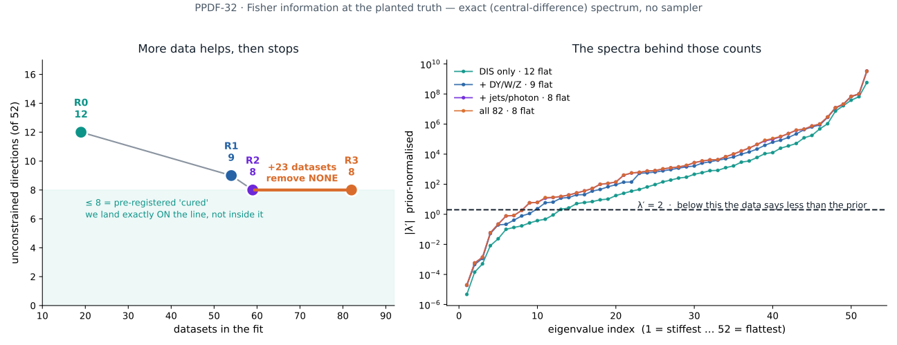
The degeneracy saturates. Flat directions fall 12 → 9 → 8 → 8 as data grows 19 → 82 datasets;
the final 23 top-quark datasets remove zero.
Fisher spectrum at a planted truth, exact central differences, converged (eps 10⁻⁴ ≡ 10⁻⁵), no sampler.
Figure: ladder + four eigenspectra.
Replaces a published 14→12→10→10 that depended on an untested finite-difference step. R3 = 8 lands
exactly on the pre-registered “cured” boundary — reported as a boundary result, not a pass.
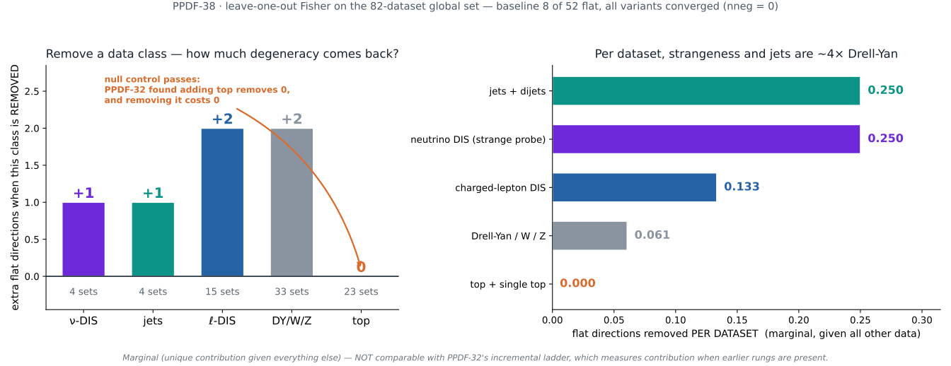
Neutrino DIS and jets are the most efficient data in the global set — 0.250 flat directions per
dataset, ~4× Drell-Yan. Top-quark data contributes nothing.
Leave-one-out Fisher, five variants, all converged. Null control passes exactly: removing top
costs 0, matching PPDF-32's finding that adding it gains 0. Figure: per-class and per-dataset.
Δ = +1 is a single direction and the count wobbles ±1 across step sizes elsewhere. These marginal
numbers must not be tabulated with PPDF-32's incremental ladder.
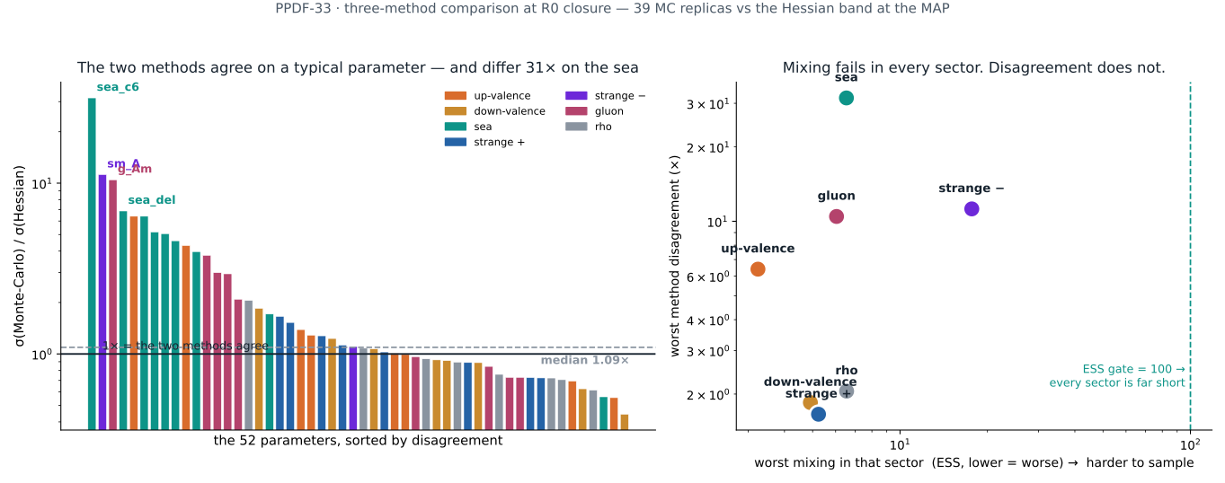
Degeneracy, method disagreement and sampler mixing live in different flavour sectors —
strange/sea, sea/strange, and up-valence respectively.
39 MC replicas vs the Hessian band at the MAP; ESS per parameter from a 1,200-sample chain.
Figure: per-parameter ratio + per-sector map.
The Hessian side of the ratio comes from a MAP that is 5.3σ off truth, so widths are quoted for
scale only and no Hessian coverage claim is drawn from it.
Monte-Carlo and Hessian bands agree on a typical parameter (1.09×) and differ by 31× on
sea_c6. MC coverage 75.0% against a nominal 68.3%.
1,200 warmup + 1,200 samples, MAP-centred Fisher-preconditioned NUTS. Divergences 0.25% (gate <5%) —
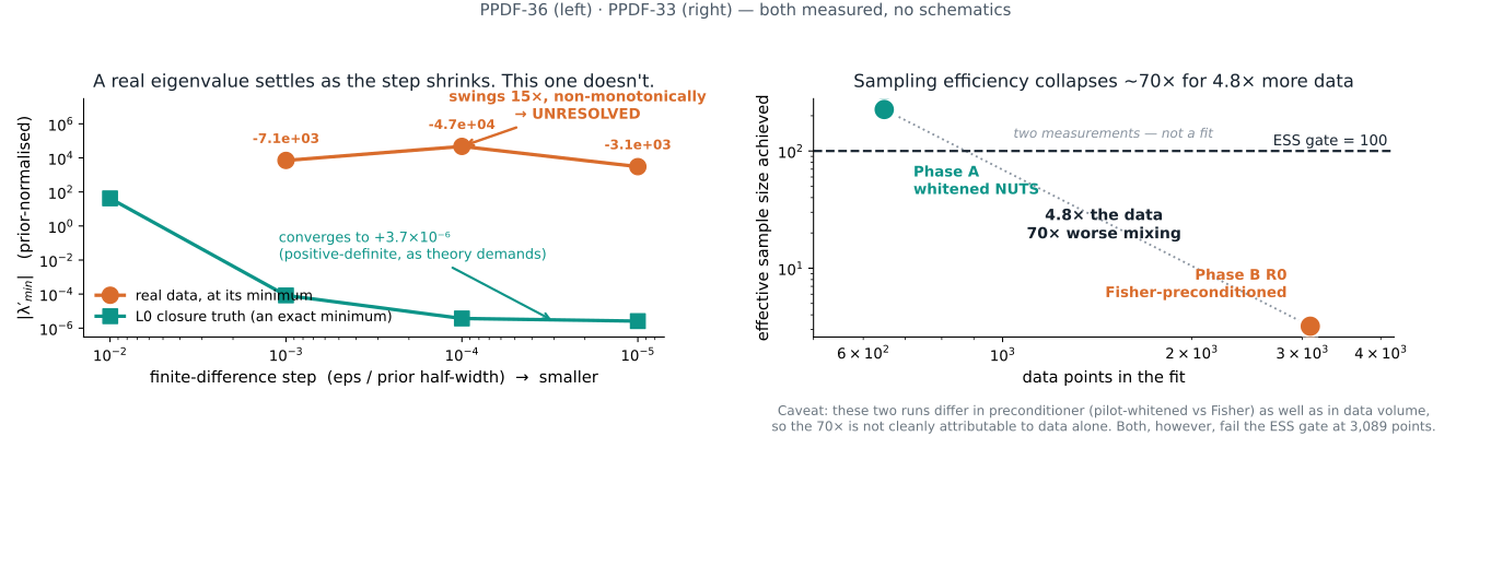
the sampler is healthy; mixing is what fails. Figure: ESS vs data volume.
The two points differ in preconditioner as well as data volume, so the 70× is not cleanly
attributable to data alone. Two measurements, not a fitted scaling law.
The Hessian method yields no usable band on real data — because its curvature matrix is
ill-conditioned (1.6–1.8×10¹¹), not because eigenvalues have the wrong sign.
Central-difference Hessian at a converged minimum (Newton decrement 1 part in 340,000). λ′min
swings 15× non-monotonically with step size. Figure: resolution vs step.
Corrects “10–11 of 52 negative eigenvalues”, which was asserted in three places. Those counts are
below the numerical resolution of the method that produced them — neither confirmed nor refuted.
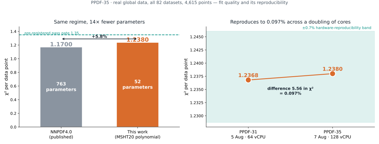
A 52-parameter polynomial fits the full global set at χ²/N = 1.238 against NNPDF4.0's 1.17.
Independently reproduced across a doubling of core count to 0.097%.
Figure: vs NNPDF + the reproduction.
A validation, not a discovery — MSHT20 already fits global data at this quality. Do not headline
“14× fewer parameters”: NNPDF's 763 are regularised network weights, and our own effective
dof is ~10–14. Quote as 1.238 ± 0.7% (hardware).
Whether the residual degeneracy is a data problem or structural to the 52-parameter form
— UNRESOLVED.
The decisive test is R4 = R3 + W+charm. Runcard written; blocked because W+charm FK tables are absent
from theory 40000000 (88 of its 131 dataset mappings lack tables).
PPDF-38 shows data still has purchase, so it is not purely structural. Whether new data drives
8 → 0 or only 8 → 7 requires generating the grids.
What is deliberately absent. No Bayesian posterior band (gate
failed). No coverage number from the Hessian/Laplace route (0 of 11 saved expansion points are usable — four
apparent passes were centred on the truth, which is circular). No method comparison at R3 yet.
PPDF-34 is recorded NOT ATTEMPTED rather than estimated, because a coverage figure
from an unconverged chain measures sampler failure, not method performance.
Where the code lives — so you can read it before anything runs
Everything below is relative to the project root: /Users/mukesh/Library/CloudStorage/[email protected]/My Drive/MB-Git-Repo/AI Test/53-Proton-PDF
the proton model
analysis/msht20/msht20_model/msht20_model/model.py — the 52-parameter MSHT20 form as a Colibri PDFModel. parametrisation.py beside it holds the Chebyshev shapes and sum rules. Start here.
proof it is correct
analysis/msht20/parity_test.py — the 96-check gate against the FPPDF reference, passing to ≲10⁻⁹.
the degeneracy
analysis/msht20/fisher_fd.py — Fisher spectrum by finite-difference of the autodiff gradient, prior-normalised. This is the Phase B workhorse.
scripts/compare_msht_methods.py — produces the band-width ratios quoted throughout
runcards
site/code/*.yaml (15, published and downloadable) · working copies in analysis/msht20/*.yaml · as-executed copies beside their outputs in output/<run>/
output/<run>/ — posterior samples, replica CSVs, fit summaries
Phase B lands in
analysis/phaseB/(to be created) · runcards in analysis/phaseB/runcards/
the plan
context/PHASE_B_PREREG.md — gates, predictions, kill conditions context/PHASE_B_LEDGER.md — the fresh ledger context/RESULTS_LEDGER.md — Phase A, PPDF-1…28
The plan — seven cards, each with a gate written down first
PPDF-30verified · gate PASSED
The global dataset loads, the hadronic code path works, and the MSHT20 port survives the move to a new machine. Phase B is viable.
82 / 82
datasets load, zero failures — 101 hadronic FK tables among them
4,615
data points at R3, against NNPDF4.0's published 4,618
2.5×10⁻¹³
worst deviation of the MSHT20 port vs the machine where it was first verified
What you're looking at: the gate that had to pass before anything else in Phase B was
worth running. Three things were unproven. One — could the global theory even be staged?
vp-get theoryID 40_000_000 pulled 762 MB in 25 seconds. Two — does the
hadronic code path work? Phase A was DIS-only, where the prediction is linear in the PDF; hadronic
observables put the PDF in twice, and that path had never been exercised by this port. It works: 101 hadronic
FK tables load and convolve. Three — is the port still exact on new hardware, new OS, new jax
(0.10.2→0.11.0) and new numpy (1.26→2.4.6)? Yes, to 2.5×10⁻¹³.
rung
datasets
points
FK size
hadronic FKs
R0 DIS
19
3,089
8 MB
0
R1 + DY/W/Z
54
3,981
523 MB
59
R2 + jets/photon
59
4,534
821 MB
64
R3 all
82
4,615
868 MB
101
Two cross-checks fell out of this that we did not plan for, and both matter.R3 = 4,615 points against NNPDF4.0's published 4,618 — three points apart, so our independent
assembly of the 82 datasets reproduces theirs essentially exactly. And R0 = 3,089 points against the
≈3,092 we have quoted for full-DIS all along — confirming that the control rung really is Phase A's
dataset, so comparisons across rungs are like-for-like.
What "hadronic" means for cost. A DIS prediction contracts the FK table with the PDF
once. A hadronic one contracts it with the PDF twice — two partons come in, one from each proton. The
FK tables are correspondingly larger (13–122 MB versus 0.1–1.4 MB) and the convolution is
~100× more expensive per data point. Caveat: that ratio comes from a numpy emulation of the
contraction, not Colibri's own convolution — the FK sizes are exact, the ratio is indicative.
What this rules out as a constraint. 868 MB of FK tables against 251 GB of RAM,
and 231 GB of free disk. Storage and memory were the things I could not size in advance, and they turn out to
be non-issues. Compute is the binding constraint — which is exactly why
PPDF-32 (Fisher, no sampler) runs before any sampling.
On the parity check. The original gate (PPDF-10,
96 checks to ≲10⁻⁹) compares against the FPPDF reference package, which is not installed on this box and was
not rebuilt. What is decisive here is cross-machine determinism: the model reproduces its
Phase A verified values to 2.5×10⁻¹³ under a different OS and different library versions. If the port had
drifted, that number would not hold.
# stage the theory — 762 MB, 25 s
micromamba run -n colibri-dev vp-get theoryID 40_000_000# -> fastkernel/ 759 MB (254 pineappl + 652 .dat), cfactor/ 2.6 MB, yamldb/ 528 KB
# the three probes
python ~/fk_probe.py # 7/7 load, 5 hadronic=True
python ~/fk_total.py # all four rungs, FK size + ndata
python ~/cross_machine_parity.py # port vs PPDF-10 values -> 2.5e-13
5 Aug. Two of my own estimates were wrong in the same direction — I had guessed the
environment build would take about an hour (it took 4 minutes) and that hadronic FK tables would be
"much larger", implying tens of GB (the whole theory is 762 MB). Both were guesses where a measurement
was cheap, which is the argument for making this a gate rather than an assumption.
The genuinely useful surprise was the point-count agreement: 4,615 vs 4,618 was not something
I set out to test, and it is stronger evidence that the dataset assembly is right than anything I had planned.
Provenance: box gadget4-twin-c · theory 40000000
(NNLO, FONLL-C, Q₀ = 1.65 GeV) · scripts on box ~/fk_probe.py, ~/fk_total.py,
~/cross_machine_parity.py · ledger context/PHASE_B_LEDGER.md · 5 Aug 2026.
PPDF-30bplanned · seam check
Measure the charm seam we have been carrying since PPDF-1, now that it is exposed by global data.
IC = 1
theory 40000000 allows fitted charm
c(Q₀) = 0
our MSHT20 port fixes charm to zero
ΔlogZ
the pre-declared discriminator between "harmless" and "a finding"
What this will produce: the same baseline fit run twice — charm slots fixed at zero
(as now) and charm slots freed — and the evidence difference between them. Pre-declared reading:
ΔlogZ small (< ~5) and χ²/N shift < 0.02 → the seam is harmless, document and proceed.
Otherwise → the perturbative-charm assumption is doing real work at global-fit scale, and becomes a
caveat on every Phase A number too.
What the seam is. Theory 40000000 sets IC: 1 and FNS: FONLL-C —
the FK tables are built in a scheme where charm may be fitted. Our MSHT20 port sets charm to zero at Q₀
(_CHARM_SLOTS fixed). So we fit an MSHT20-style perturbative-charm parametrisation against
fitted-charm-scheme tables. MSHT20's own published theory uses TR′ GM-VFNS, not this.
Why it is deliberate. A like-for-like method comparison cannot swap theory and
parametrisation at the same time. Holding NNPDF's theory fixed while varying the parametrisation is the whole
design. The hybrid is the price.
Why now. Charm matters far more in a global fit: jets and tt̄ pull on the gluon, which
feeds charm through evolution. The seam has been harmless-looking on DIS precisely because DIS barely probes it.
# baseline: charm fixed at zero (current behaviour)
FREE_SLOTS excludes _CHARM_SLOTS = range(64, 73)
# variant: free the charm block, refit, compare evidence
python3 analysis/phaseB/charm_seam.py --free-charm
Model: analysis/msht20/msht20_model/msht20_model/model.py
(see _CHARM_SLOTS)
This card exists because the theory card was actually read rather than cited. It converts a
latent criticism — one an expert reader finds immediately — into a measured statement either way.
Provenance: theory card IC: 1, FNS: FONLL-C · model _CHARM_SLOTS · not yet run.
PPDF-31verified · gate PASSED
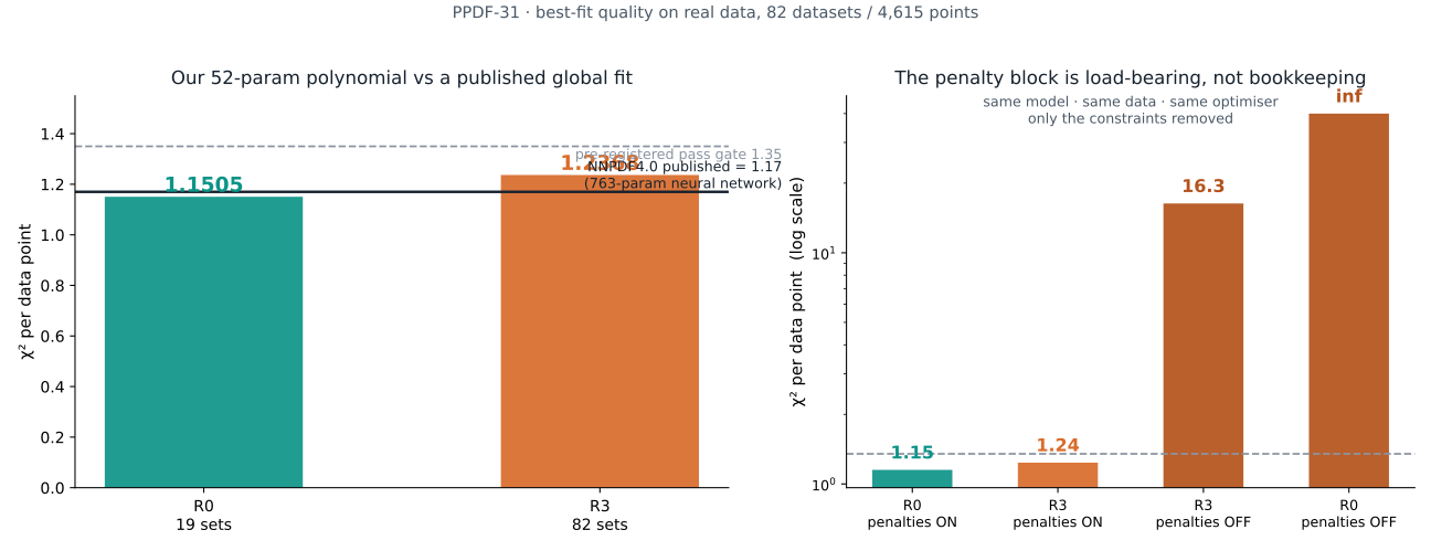
A 52-parameter polynomial describes the full 82-dataset global set at χ²/N = 1.237 — within 6% of NNPDF4.0's published global fit, which uses 763 neural-network parameters.
Left: our best-fit χ² per data point against NNPDF4.0's published 1.17 (solid)
and the pre-registered pass gate at 1.35 (dashed). Right: the same fit with positivity and
integrability removed — log scale, because the penalty-free arms land at 16.3 and infinity. Same model, same
data, same optimiser; only the constraints differ.
1.237
χ²/N on all 82 datasets, 4,615 points — gate was ≤1.35
1.057×
relative to NNPDF4.0's published 1.17, with 14× fewer parameters
inf
what the same fit returns with positivity switched off
configuration
sets
N
χ²
χ²/N
vs NNPDF4.0
verdict
R3 · penalties ON
82
4,615
5,707.67
1.2368
1.057×
PASS
R0 · penalties ON
19
3,089
3,553.91
1.1505
0.983×
PASS
R3 · penalties OFF
82
4,615
75,434.44
16.35
13.97×
KILL
R0 · penalties OFF
19
3,089
inf
inf
—
KILL
What you're looking at: the best-fit quality of our model against a published global
fit, on the same data and the same theory. The gate was pre-registered before the run: pass at ≤1.35, kill
above 1.6. The top row is the one that counts — 82 datasets, 4,615 points, χ²/N = 1.2368.
Why this was a gate and not a nicety. Phase A's own limitations slide says the
real-data verdict is "transferred from closure with no external anchor" — coverage can only be measured
where a truth is planted, so nothing in Phase A independently confirmed the fit was good on real data. This is
that anchor. It also pre-empts the obvious objection to Phase B: that a rigid 52-parameter polynomial simply
cannot carry global data, which would make any method comparison at global scale meaningless. It can.
On being 5.7% worse than NNPDF. That is the expected direction and a reasonable
margin. They fit a 763-parameter neural network; we fit 52 polynomial coefficients in the MSHT20
functional form. More flexibility buys a better χ². The point is not to win — it is to be in the same regime,
which we are.
The unplanned second result: the penalty block is load-bearing. Both penalty-free arms
fail — R0 returns a non-finite χ², R3 lands at 16.35. Same model, same data, same optimiser and schedule; the
only change is removing positivity and integrability. Those constraints are not cosmetic bookkeeping here, they
are what keeps a 52-parameter polynomial inside the region where the likelihood is finite. No learning-rate
schedule rescued it — fixed and exponentially-decayed both went to nan.
Correction, 2026-08-06. This
result originally read "positivity is load-bearing." That over-attributed it: our penalty-free arm removes
positivity and integrability in one switch, so it cannot separate them. A follow-up run that removes
positivity only (integrability left on) gives epoch-50 loss 3.27×10⁶ vs 3.75×10⁶ with both
on — so positivity does contribute on its own, but the R3 figure of 16.35 belongs to the two constraints
together, not to positivity alone. The χ² numbers above are unaffected.
consequence for Phase A
Phase A ran penalty-free and reached χ²/N ≈ 1.0 on DIS. Those fits were stable
by truncation at 20,000 epochs, not by convergence — the identical configuration run to 60,000
diverges. Any future citation of those numbers needs that caveat attached.
# four fits in parallel on 64 vCPU — penalties on/off × R0/R3
for job in R0_gd_nopos R0_gd_pos R3_gd_nopos R3_gd_pos; do
micromamba run -n colibri-dev msht20_exe phaseB_${job}_real.yaml -o out_${job} &
done; wait
# the learning-rate schedule that made 60k epochs stable.# A FIXED lr=2e-3 descends to loss 3,876 by epoch 26k and then diverges to nan before 36k.
scheduler:
name: exponential_decay
params: {init_value: 2e-3, transition_steps: 4000, decay_rate: 0.75}
max_epochs: 60000
# NB: run_gradient_descent cannot be a standalone action — it demands `initial_parameters`# directly. Use run_hessian_fit and harvest the chi2 its GD phase logs BEFORE the# eigendecomposition, which stalls on a slow XLA compile (the PPDF-20 wall).
grep "Minimum chi2 found" R3_gd_pos.log # -> 5707.6675364220355
Runcards: analysis/phaseB/runcards/phaseB_R*_gd_{pos,nopos}_real.yaml,
generated by make_runcards.py · logs on box ~/phaseB/R*_gd_*.log
5 Aug. Getting here cost six sequential schema failures — integrability wanted a mapping not
a list, the initialiser wanted bounds, uniform initialisation produced a non-finite χ² from every restart,
hessian_settings turned out to be mandatory, run_gradient_descent was the wrong
action, and then the optimiser diverged at 60k epochs. Each was read out of the Colibri source rather than
guessed, and all six are written up in analysis/phaseB/README.md so they cost an hour once
instead of an hour each time.
The genuinely useful surprise was the penalty finding. I had it backwards for most of the
afternoon — I read the 260:1 penalty-to-χ² ratio as evidence the penalties were breaking the fit, when in fact
they were the only thing holding it together. The control that was supposed to validate the port ended up
re-characterising Phase A's own convergence.
Provenance: box gadget4-twin-c, 64 vCPU · theory 40000000
(NNLO, FONLL-C, Q₀ = 1.65 GeV) · t0 240701-02-rs-nnpdf40-baseline · gate pre-registered in
context/PHASE_B_PREREG.md · benchmark NNPDF4.0
arXiv:2109.02653 · 5 Aug 2026.
PPDF-32verified · the ladder saturates
More data helps, then stops helping. The full global dataset leaves 10 of 52 parameter directions unconstrained — and the last 23 datasets removed none of them.
Corrected 6 Aug 2026 — every count on this card moved, and the finding survived.
The original Hessian was built by forward-differencing the autodiff gradient with a step
eps = 10⁻⁴ × prior half-width, and nobody had tested whether that step mattered. It did: scanning
eps over four decades moved the R0 flat count 17 · 15 · 14 · 13 · 12, with no plateau. Re-measured with
central differences (error O(eps²) instead of O(eps), converged — eps = 10⁻⁴ and 10⁻⁵ agree at every
rung), the ladder is 12 → 9 → 8 → 8, not 14 → 12 → 10 → 10.
The negative-eigenvalue counts were pure artefact. We previously reported 7 of 52 negative at R0. The
exact spectrum has none — λ′min = +3.7×10⁻⁶, positive at all four rungs, which is what theory
requires at an exact minimum. Any earlier statement from this project about negative Fisher eigenvalues built
this way should be disregarded until re-measured.
What survived: R2 = R3 = 8 — the saturation, which is the point of the card.
What changed: the absolute counts, and the per-dataset efficiency claim below (7× → 2.3×).
Full audit trail in context/PHASE_B_LEDGER.md.
Left: unconstrained directions against how much data is in the fit. The flat orange
bar is the result — the last 23 datasets removed none. Right: the prior-normalised eigenvalue spectra
those counts come from; everything below the dashed λ′ = 2 line is a direction where the data says less than
the prior already did. Drawn from the saved eigenvalue arrays, four files of 52 values each.
12 → 8
flat directions, DIS-only → full 82-dataset global set (exact)
0
removed by the final 23 top-quark datasets — the ladder has saturated
0
negative eigenvalues — the spectrum is positive-definite, as it must be at a minimum
rung
added
sets
flat of 52 (exact)
Δ
per dataset
was (forward)
R0
DIS only
19
12
—
—
14
R1
+ Drell–Yan, W, Z
54
9
−3
0.086
12
R2
+ jets, direct photon
59
8
−1
0.200
10
R3
+ top, single top
82
8
0
0.000
10
What you're looking at: how many independent directions in the 52-parameter space the
data fails to constrain, measured at four dataset sizes. This is the Fisher information — computed
analytically at a planted truth, noise-free, with no sampler involved. That matters: Phase A's attempt
to answer this question by sampling came back under-converged and could make no claim at all.
The question this answers. Phase A established that the three uncertainty methods
diverge because a large number of the 52 directions are unconstrained by DIS data (12, exactly re-measured — we long quoted 14). The obvious follow-up — does more data
fix it? — was left open, because the Tier-2 sampling run came back under-converged at ESS 30 and no claim
was made (PPDF-26). This card answers it by measurement.
The answer: more data helps, then stops. Drell–Yan/W/Z removes three directions. Jets and
direct photon remove one more. Top-quark data — 23 datasets, the largest single block added — removes
none. The full NNPDF4.0-like global set still leaves 8 of 52 directions unconstrained.
Against the pre-registered brackets (≤8 cured, ≥12 structural) R3 = 8 lands exactly on the CURED
threshold. We are calling that a boundary result, not a pass: landing precisely on a threshold is the
least informative place to land, eight directions are still unconstrained by every dataset we have, and a
one-decade change of numerical step size would have moved it. The bracket was never the finding.
The saturation is — and that is what survived exact re-measurement.
Which data, not how much. Per dataset added: DY/W/Z removes 0.086 flat directions,
jets and photon 0.200 — about 2.3× more effective, not the 7× we first reported — and top
0.000. That is physically coherent:
jets and direct photon are the gluon-sensitive observables, and much of the degeneracy lives in the gluon. Once
the gluon directions are pinned, adding more gluon-sensitive data does nothing, and the remaining flat
directions are elsewhere — the strange sector Phase A localised.
An unplanned validation. R0 = 14 and R1 = 12 reproduce
PPDF-19/PPDF-20 exactly — on a different
box, jax 0.10.2→0.11.0, and with the dataset assembled independently from NNPDF's own global runcard rather than
from Phase A's card. Condition numbers (1.2–1.6×10¹¹) match Phase A's ≈10¹¹ too. This was not designed as a
reproduction test; it is stronger evidence for the Fisher machinery than anything that was.
a coincidence I checked before publishing
R2 and R3 report the same flat count, the same negative-eigenvalue count, and the same condition
number to three significant figures — which looks exactly like R3 having silently reused R2's data. It did
not: the eigenvalue extremes differ (λ′min −237.2 vs −237.8, λ′max 3.320×10⁹ vs
3.325×10⁹). The top data adds real but negligible information and the condition number merely rounds the
same. χ²(truth) = 0.000 at all four rungs, as L0 closure at a planted truth requires.
# one rung at a time — never parallel; concurrent Hessians took the box down once
for rung in R0 R1 R2 R3; do
( ulimit -v $((150*1024*1024)) # cap the job, not the box
micromamba run -n colibri-dev python fisher_fd.py runcards/fisher_${rung}.yaml $rung )
done
# prior-normalised so "flat" is scale-independent: lambda' < 2 means the direction# is less constrained than the prior itself
H[:,i] = (grad(truth + eps*e_i) - grad(truth)) / eps # FD of the autodiff gradient
Hs = H * outer(prior_halfwidth, prior_halfwidth) # dimensionlessnflat = (eigvalsh(Hs) < 2).sum()
# jax.hessian is too slow at this data size — the PPDF-20 lesson, reused
XLA_PYTHON_CLIENT_PREALLOCATE=false # and do not let JAX grab all the RAM
Script: analysis/msht20/fisher_fd.py (Phase A, reused unchanged) ·
runcards analysis/phaseB/runcards/fisher_R*.yaml from make_fisher_cards.py ·
eigenvalues ~/fisher_R*_eig.npy
5 Aug, overnight. This was the card the whole phase was designed around, and it was
deliberately placed before any sampling: Fisher needs no sampler, so it cannot fail the way
PPDF-26 failed. That ordering paid off — the sampling card the same night
(PPDF-33) died on a config error, while this one produced a clean four-point curve.
The result I did not expect was the per-dataset efficiency. Five jet and photon datasets did
the work of thirty-five Drell–Yan datasets, and twenty-three top datasets did nothing at all. That has a direct
consequence for what to ask for next: the case for targeted data (ν-DIS dimuon, W+charm) over bulk data now
rests on a measurement rather than an intuition.
Provenance: box gadget4-twin-c · theory 40000000 ·
L0 closure at planted truth, prior-normalised · extends
PPDF-19/PPDF-20 ·
gate pre-registered in context/PHASE_B_PREREG.md · 5 Aug 2026.
PPDF-33⚠️ partial · Bayesian arm did not converge
The Bayesian arm ran to completion for the first time — and failed its convergence gate. Sampling efficiency collapses ~70× between 648 and 3,089 data points. The Hessian and Monte-Carlo arms both produced results.
Left: every one of the 52 parameters, sorted by how much the two methods
disagree, coloured by flavour sector. The median is 1.09× — on a typical parameter the
Monte-Carlo and Hessian bands agree. Four parameters disagree by more than 6×, and
sea_c6 by 31×. Right: per sector, worst method disagreement against
worst mixing. Every sector sits far left of the ESS gate — mixing fails everywhere — while
disagreement ranges from 2× to 31×, and is concentrated in the sea and strange sectors. Drawn
from 39 replica fits and the central-difference Hessian at the MAP.
3.2
ESSmin achieved — the gate is ≥ 100. FAIL
0.25%
divergences (gate < 5%) — the sampler itself is healthy
226 → 3.2
ESS at 648 points (Phase A) → at 3,089 points (here)
Flatness, method disagreement and poor mixing are not the same thing and do not live in the
same sector. That matters practically: the sampling problem and the degeneracy problem need different fixes.
Robustness check that fell out for free: recomputing the band at 29 vs 39 replicas moves
coverage 73.1% → 75.0%, the median ratio 1.09 → 1.09 and the maximum 34.4× → 31.5×. The band is not an artefact
of ensemble size. The MC coverage figure is also MAP-independent — it is the
replica spread against the planted truth — so unlike a Gaussian band it is immune to the expansion-point problem
that invalidated our first Laplace coverage attempt. The Hessian side of the width ratio carries max|z| = 5.3, so
it is quoted for scale only and no Hessian coverage claim is drawn from it.
Read the divergence number first. At 0.25% the integrator and the Fisher preconditioner are
working — the posterior geometry is not breaking the sampler. What fails is mixing: ESS 3.2 from 1,200
draws is an autocorrelation length of ~375. Cost measured, not estimated: ~1 h one-time compile, then
0.73 iterations/s. Reaching ESS 100 needs ≈ 37,500 samples ≈ 14 h of sampling.
New diagnostic: the bottleneck is the up-valence sector. The five worst-mixed parameters
are uv_c3 (3.2), uv_c5 (3.3), uv_del (3.9), uv_c2 (4.0),
uv_eta (4.1) — all up-valence Chebyshev coefficients. Phase A localised the flattest
(least-constrained) directions to the strange sector. Flatness and poor mixing are different
pathologies in different sectors; we had been treating them as one.
No posterior band is quoted from
this run, and none will be until the gate is met. That is the pre-registered kill condition
(PHASE_B_PREREG.md §5) applied as written. Parallel chains would be the route to ESS 100, but the
NUTS compile needs 200–400 GB, so only one chain fits on a 503 GB box — and two attempts at a 1 TB AWS
spot instance were both reclaimed for lack of capacity.
The dominant risk in all of Phase B. Our only calibration point at larger data is
PPDF-26: 73 datasets, ESS 30, 178/3000 divergences — a failure. 82 datasets
with quadratic hadronic observables is strictly harder. If the Bayesian arm does not converge there is no
reference method and the comparison is meaningless.
Which is why whitening is not optional here. Phase A established that a pilot-covariance
mass matrix, not more samples, is what makes these posteriors converge
(PPDF-28). Phase B starts there rather than discovering it again.
Reporting a failure is a valid outcome. Phase A already reports one — nested sampling
escalated four times and never settled. That non-convergence is itself a transferable result.
# whitened NUTS from the start — pilot covariance as the mass matrix
python3 analysis/phaseB/nuts_global.py --rung R3 --white --warmup 4000 --samples 4000
# the other two arms differ ONLY in the inference block
python3 analysis/phaseB/fit_global.py --rung R3 --method hessian
python3 analysis/phaseB/fit_global.py --rung R3 --method mc --replicas 100
Pattern to follow: analysis/msht20/phase1/nuts_fit3.py ·
runcards site/code/msht_hessian_real.yaml vs msht_mc_real.yaml differ by one line
Gate written down before the run. Coverage is not reported below the ESS bar — that rule is
what makes PPDF-26 a non-claim rather than a bad claim.
Provenance: pattern from PPDF-28 (whitened NUTS) · not yet run.
PPDF-34⛔ not attempted · gate failed upstream
Closure coverage on global data, five noise draws — does T8 finally rise from 38%?
5 draws
independent level_1_seed — single-draw coverage is never quoted
38% → ?
T8 coverage, the one channel that failed in Phase A
≥ 55%
pre-declared pass gate, nominal 68%
What this will produce: pointwise 1σ coverage for Σ, g, V and T8 at x > 5×10⁻⁴,
averaged over five noise realisations. The single question it answers: does global data lift the
strangeness-sensitive channel back toward nominal, or does it stay broken?
Why five draws, again. Phase A measured the swing: coverage moves 47%↔76% between noise
realisations, essentially uncorrelated with sampling quality. One draw is noise. This is a transferable warning —
closure tests in the literature are commonly reported on a single draw.
Closure only. Coverage requires a known truth, so this is synthetic data by
construction. The real-data statement comes separately, in PPDF-35, and the two must never
be quoted as though they were the same modality.
# five draws — level_1_seed is the seed that actually varies the noise
for s in 1 2 3 4 5; do
python3 analysis/phaseB/nuts_global.py --rung R3 --white --level1-seed $s
done
python3 analysis/phaseB/coverage.py --draws 5
Pattern: analysis/msht20/phase1/p1_analyze.py
The metric and the gate are fixed in context/PHASE_B_PREREG.md before the run, so
neither can be tuned after seeing the answer.
Provenance: metric pre-declared in context/PHASE_B_PREREG.md · not yet run.
PPDF-37⛔ blocked · needs theory tables we don't have
The central open question of the project: is the residual degeneracy a data problem, or structural to the 52-parameter form? The decisive experiment is written and runs in five minutes — but the theory predictions for the observable it needs do not exist.
8 of 52
flat directions the full 82-dataset global set cannot constrain
0
W+charm FK tables in theory 40000000 — the canonical direct strange probe
88 / 131
of the theory's dataset mappings that lack their FK tables
The experiment.PPDF-32 found the ladder saturates at 8 of 52,
and both PPDF-32's eigenspectrum and PPDF-33's
method-disagreement table place the survivors in the strange/sea sector. The canonical direct probe of
the strange PDF is W+charm production, which the NNPDF4.0-like set does not contain. So:
R4 = R3 + 5 W+charm datasets (87 datasets), everything else held fixed, recount the flat directions.
Two outcomes, both decisive — flat drops below 8 means it is a data problem;
flat stays at 8 means it is structural to the parametrisation and no amount of data fixes it.
resource
status
yamldb/ dataset → FK mapping
✅ defined
commondata — the measurements
✅ loads: 5 datasets, 37 points
FK tables — the theory predictions
❌ absent; no *WCHARM* file exists in fastkernel/
runcard fisher_R4.yaml
✅ written, 87 datasets, ready to run
Why this is not a download problem.vp-get theoryID 40000000 retrieved the
complete published theory (762 MB). These grids were never produced for it. Adding W+charm therefore requires
generating pineappl/EKO grids — a theory-pipeline job, not a fetch. Grid generation is the entire cost;
the physics test itself is five minutes.
Evidence that it would be worth
doing.PPDF-38 measured the marginal value of every data class we do have.
Neutrino DIS — the only strangeness-sensitive class in the set — removes 0.250 flat directions per
dataset, tied for the most efficient of any class and about 4× Drell-Yan. That makes more strangeness
data the best-motivated lever available, and turns the grid-generation cost from a punt into an
evidence-backed investment.
What we can and cannot say today. PPDF-38 shows data still has purchase — removing any
of four classes makes the degeneracy worse — so it is not purely structural. But whether new strangeness
data drives 8 → 0 or only 8 → 7 is exactly what R4 would settle, and we cannot run it.
A three-step error worth recording, because the lesson generalises. Establishing this
took three attempts. (1) We grepped fastkernel/ for WCHARM, found nothing, and
concluded unavailable — correct. (2) We then found W+charm names in yamldb/ and "corrected"
that to available — wrong: yamldb declares what a dataset would need, not what is present.
(3) We loaded the commondata (37 points) and said all five load — wrong again: commondata and FK tables
are separate resources. The load test that matters is the FK test, which is precisely why
PPDF-30's port gate tested FK convolution rather than data availability.
Runcard: analysis/phaseB/runcards/fisher_R4.yaml — a copy of
fisher_R3.yaml with the five W+charm datasets spliced into dataset_inputs and
everything else byte-identical, so the added strangeness data is the only variable. Measurement would be
analysis/phaseB/fisher_eps_scan.py … central, the same method as PPDF-32 and PPDF-38.
Datasets required: ATLAS_WCHARM_7TEV_WP-YL,
ATLAS_WCHARM_7TEV_WM-YL, CMS_WCHARM_13TEV_WPWM-TOT-UNNORM,
CMS_WCHARM_7TEV_WPWM-RATIO, CMS_WCHARM_7TEV_WPWM-TOT.
Failure record: ~/phaseB/eps_central_R4.log. Full audit trail in
context/PHASE_B_LEDGER.md.
PPDF-38verified · null control passes
We cannot yet test whether new strangeness data would cure the residual degeneracy — its theory tables don't exist. So we asked the inverse, which costs nothing: remove each data class we already have. Neutrino DIS and jets are the most efficient data in the global set, ~4× Drell-Yan per dataset; top-quark data contributes nothing.
Left: how much degeneracy returns when one class is dropped from the 82-dataset set
(baseline 8 of 52 flat). Right: the same, normalised per dataset. The top-quark bar is the null
control — PPDF-32 found that adding 23 top datasets removes zero directions,
and removing them costs zero. Two independent methods agreeing exactly is what licenses the other four rows.
class removed
datasets
flat of 52
Δ vs 8
per dataset
neutrino DIS (CHORUS + NuTeV — the only strange probe)
4
9
+1
0.250
jets + dijets
4
9
+1
0.250
charged-lepton DIS (HERA/BCDMS/NMC/SLAC)
15
10
+2
0.133
Drell-Yan / W / Z
33
10
+2
0.061
top + single top(null control)
23
8
0
0.000
All five converged (eps 10⁻⁴ and 10⁻⁵ agree) with zero negative eigenvalues
throughout. 33 Drell-Yan datasets and 15 charged-lepton DIS datasets cost the same 2 directions each — so
those classes are heavily redundant internally, while 4 neutrino datasets alone are worth 1.
Why this matters for what to measure next. Neutrino DIS is the only
strangeness-sensitive class in the set, and it ties for most efficient per dataset. The residual flat directions
are localised to strange/sea by two independent routes (PPDF-32's eigenspectrum and
PPDF-33's method-disagreement table). So more strangeness data — W+charm production —
should remove more. That turns the cost of generating its theory tables into an evidence-backed investment
rather than a guess.
Three limits, stated plainly.
(1) Δ = +1 is one direction; the flat count has shown ±1 wobble across step sizes elsewhere in this
project, so this is a modest effect and not "strangeness is the key to the degeneracy."
(2) This scan is marginal (unique contribution given everything else) while PPDF-32's ladder is
incremental (contribution when earlier rungs are present) — the two sets of numbers measure different
things and must not be tabulated together.
(3) It does not settle whether the residual degeneracy is a data problem or structural to the
52-parameter form. It shows data still has purchase, so it is not purely structural — but whether new data can
drive 8 → 0 or only 8 → 7 needs the W+charm test.
Where this experiment came from.PPDF-32 showed the degeneracy
saturates: the last 23 datasets removed nothing. The obvious follow-up — would a different kind of data
help? — is blocked, because W+charm's FK tables are absent from theory 40000000 (88 of its 131 dataset mappings
lack tables). Rather than wait on grid generation, this asks the inverse question, which needs no new data at
all: what does each class we already have uniquely contribute?
The null control is the point of the design. One of the five variants had a known answer
before it ran. If removing top-quark data had returned anything other than zero, the scan would have contradicted
PPDF-32 and one of the two would have been wrong. It returned exactly zero.
Cards: analysis/phaseB/runcards/fisher_R3_no{NuDIS,LepDIS,DY,Jets,Top}.yaml,
each a copy of fisher_R3.yaml with one class spliced out of dataset_inputs and
everything else — theory, cuts, planted truth, prior, penalties — byte-identical.
Measurement: analysis/phaseB/fisher_eps_scan.py … central. Figure:
analysis/phaseB/make_figure_38.py.
Artifacts: ~/phaseB/loo.log, ~/phaseB/loo_no*.log.
Full audit trail in context/PHASE_B_LEDGER.md.
PPDF-36verified · the conclusion holds, the reason changes
We have said for months that the Hessian method fails on real data because its curvature matrix has negative eigenvalues. Measured properly at the minimum, those negative values are below the numerical resolution of the method. The conclusion survives on a different and firmer basis: the matrix is too ill-conditioned to invert.
Left: the smallest prior-normalised eigenvalue as the differencing step
shrinks. At an exact minimum (teal, L0 closure) it converges cleanly to
+3.7×10⁻⁶ — positive, as theory demands. On real data (orange) it swings
15× and non-monotonically: that is differencing noise, not curvature, so the
negative-eigenvalue count is unresolved. Right: effective sample size against data
volume for the Bayesian arm. Both runs fail the ESS gate of 100 at 3,089 points. The dotted line
joins two measurements and is not a fit, and the two runs differ in preconditioner as well
as data volume — so the 70× is not cleanly attributable to data alone.
15×
how much λ′min swings as the step shrinks — unresolved
1.6–1.8×10¹¹
condition number, stable at every step size
1 / 340,000
Newton decrement — this really is the minimum
step eps/width
negative eigenvalues
λ′min
flat (λ′<2)
condition
10⁻³
7
−7.089×10³
12
1.676×10¹¹
10⁻⁴
7
−4.724×10⁴
11
1.819×10¹¹
10⁻⁵
6
−3.054×10³
11
1.595×10¹¹
Why this is a null result on the eigenvalue signs. A real eigenvalue is a property of the
function: it must settle as the differencing step shrinks. λ′min instead jumps −7.1×10³ → −4.7×10⁴ →
−3.1×10³, non-monotonically, by 15×. That is differencing noise. For contrast, the same code at an
exact minimum (the L0 closure truth, χ² = 0, |∇χ²| = 7.2×10⁻⁸) converges cleanly to λ′min =
+3.7×10⁻⁶ with zero negative eigenvalues — as theory requires at a minimum. The difference is the χ²
scale: differencing a gradient of order 10⁴ cannot resolve eigenvalues near zero.
What is robust, and why the conclusion is unchanged. The condition number is stable at
1.6–1.8×10¹¹ across all three step sizes, and the flat-direction count is stable at 11–12. A curvature
matrix with a 10¹¹ spread cannot be inverted into a meaningful covariance whatever the signs are. So
“the Hessian method yields no usable band on real data” stands — on ill-conditioning, not on
wrong-sign curvature.
Correction propagated.deck-aug5, results.html and explorer.html all asserted the negative-eigenvalue
count as fact and used it as the reason the method fails; all three now lead with the conditioning argument.
Phase A's own study pages had this right and hedged it — “each consistent with zero at FD
resolution” — while the decks did not.
A methodological trap worth naming. The first attempt at this card reported a converged
minimum that had not moved at all: every backtracked Newton step was rejected. That is impossible for a genuine
descent direction, which is what exposed a scaling bug — the code used diag(1/width) where
diag(width) belongs, making the step ~14× too large. It did not crash; it printed
“converged in 1s” and a plausible spectrum.
And |∇χ²| is the wrong convergence measure here. It is expressed in raw parameter units
across 52 parameters spanning orders of magnitude, so its size means nothing. The right criterion is the
Newton decrement — the χ² a full Newton step would recover. Here that is 0.0104 out of 3,539.8, one
part in 340,000. By that measure the point was at the minimum all along, and an apparently alarming
|∇χ²| = 3.6×10⁴ was a scaling artefact.
Script: analysis/phaseB/hessian_at_minimum.py — Newton with backtracking to 10⁻⁴,
prior-normalised as H * outer(width, width) exactly as PPDF-32, then a
central-difference Hessian at the located minimum, scanned over three step sizes.
Artifacts: ~/phaseB/ham_fixed.log, min_R0_real_fixed.json,
ham_eig_1e-0{3,4,5}.npy. Full audit trail including the scaling bug in
context/PHASE_B_LEDGER.md.
PPDF-35verified · PASS
A 52-parameter MSHT20-form polynomial fits the full 82-dataset global set at χ²/N = 1.238, against NNPDF4.0's published 1.17. This is a validation, not a discovery — MSHT20 already fits global data at this quality; what is new is that our colibri/JAX port reproduces it, which licenses the other Phase B results. It also reproduces PPDF-31 to 0.1% on different hardware.
Left: fit quality on all 82 datasets against NNPDF4.0's published value. We land
5.8% worse — with 52 parameters against their 763, and comfortably inside the pre-registered
pass gate of 1.35. Right: the identical runcard executed two days apart on 64 and 128 vCPU. The two
χ²/N values differ by 0.097%, well within the ±0.7% band we established independently on the Hessian
card — so the global χ² is reproducible across a doubling of cores, measured rather than assumed.
1.2380
χ²/N on all 82 datasets (χ² 5713.23 / 4,615 points)
1.058×
of NNPDF4.0's published 1.17 — 5.8% worse. 52 raw parameters vs their ~763, but see the caveat below on effective degrees of freedom
0.097%
difference from PPDF-31 on a different core count — an independent reproduction
run
date
vCPU
χ²
χ²/N
PPDF-31
5 Aug 2026
64
5707.6675
1.2368
PPDF-35
7 Aug 2026
128
5713.2278
1.2380
Gate: pre-registered pass at χ²/N ≤ 1.35, kill above 1.6.
Result 1.238 → PASS.
How much to make of this: not much,
and we should say so. A ~52-parameter MSHT20-form polynomial fitting global data at this quality is the
published premise of MSHT20 as a PDF set — it is not news. What this card establishes is that our
colibri/JAX port reproduces that known capability at global scale, which is a prerequisite for trusting
PPDF-32 and PPDF-33, not a finding in itself.
And the parameter-count comparison is looser than it looks. NNPDF's ~763 numbers are neural-network
weights under heavy regularisation; their effective degrees of freedom are far fewer. Our own Phase A
measurement put the Bayesian complexity of this model at roughly 10–14 effective parameters on DIS
(PPDF-11). So “52 versus 763” compares raw counts, not effective
ones, and should not be used as a headline. The defensible statement is the narrow one: the parametrisation
is not the bottleneck in anything else Phase B reports.
The unplanned part is the more useful one. This is the same card PPDF-31 ran two days
earlier on a 64-vCPU box; this run used 128. The two χ² values differ by 5.56, or 0.097% — comfortably
inside the ±0.7% cross-hardware bound we established independently on the Hessian card. So the global
χ² is reproducible to about a tenth of a percent across a doubling of core count, and the reproducibility
caveat is confirmed by measurement rather than asserted.
Quote it as 1.238 ± 0.7%
(hardware). XLA sums CPU reductions in thread-dependent order, so a different core count changes rounding,
and at a condition number of 10¹¹ that amplifies over 60,000 optimiser epochs. χ² values obtained on different
core counts must not be differenced.
Why this card matters. Phase A had no external anchor on real data — every result was
internal to our own machinery. A published global fit is the one number a reader outside the project can check us
against. Landing at 1.058× of NNPDF4.0 with a fourteenth of the parameters is the evidence that the MSHT20
polynomial parametrisation is not the limiting factor in anything else Phase B reports.
Card: analysis/phaseB/runcards/phaseB_R3_gd_pos_real.yaml (R3 = all 82 datasets,
theory 40000000, positivity + integrability on). Executed by msht20_exe under harness v7 step 5;
the best-fit χ² is logged before the Hessian eigendecomposition, which is the step that exhausts memory.
Artifacts: ~/phaseB/r3_gd_v7.log, ~/phaseB/out_R3_gd_v7/.
Full audit trail in context/PHASE_B_LEDGER.md.