One card per registered result; IDs are immutable. Each card has four tabs:
Results (what we produced and what you're looking at), Explanation (the physics and the method),
Code (exactly how to reproduce it), Notes (the story of how it happened). Status:
verified ·
provisional (caveats attached) ·
lesson (a failure that taught us something).
1 · Calibration — fitting planted protons whose true shape we know.
Synthetic data, real machinery: these results test the instrument, not the proton.
PPDF-1verified · replication
Clean drill passed: fed noise-free synthetic data, the fit recovers the planted proton near-exactly.
What you're looking at: three numbers, no plot — this result is the numbers.
The first says the best fit misses the 648 synthetic data points by 0.0002 of an error bar each: since the data
carried zero noise, anything much larger would have signalled a bug. The paper we're replicating quotes
χ² ~ 10⁻⁴–10⁻⁵ for this same test (Table 3.1) — we land in the same regime. The third number is a health
identity (explained in the next tab) that only holds when the sampling is behaving; here it holds to 3%.
The physics. A proton's structure is encoded in PDFs — for each parton type, x·f(x) says
how the proton's momentum is shared (wiki). Our synthetic "measurements" are
deep-inelastic structure functions F₂(x, Q²): the rate of electrons scattering off the proton at momentum
fraction x and resolution Q. Theory connects the two linearly: prediction = FK ⊗ f, where the FK table
precomputes the QCD matrix element and DGLAP evolution (wiki).
The model being fitted: the Les Houches benchmark shape — per flavour combination,
x·f(x) = A x^α (1−x)^β (1 + ε√x + γx) — 13 free parameters after sum rules. The truth was planted using this
same shape, so exact recovery is possible.
The statistics. Misfit is χ²(θ) = [D − T(θ)]ᵀ C⁻¹ [D − T(θ)] with C the experimental
covariance (t0 prescription, wiki). Bayes: posterior p(θ|D) ∝ e^(−χ²/2) π(θ), uniform
prior boxes π. Nested sampling (UltraNest, 200 live points) explores the 13-dim posterior and computes the
evidence Z = ∫ e^(−χ²/2) π dθ. On noiseless data the optimum is χ² = 0; the health identity
⟨χ²⟩ = χ²_min + complexity diagnoses honest sampling (wiki).
# environment (one-time)
micromamba create -n colibri-dev -f colibri/environment.yml
micromamba run -n colibri-dev pip install -e colibri/colibri/examples/les_houches_example
# run the fit (auto-downloads FK tables + PDF sets on first run)
micromamba run -n colibri-dev les_houches_exe lh_fit_closure_test.yaml
2 Jul, afternoon. First full flight of the machinery, and it flew on the first attempt — the
env build was the only slow part. The 8m22s wall time included downloading four decades of experimental data.
The moment we trusted the statistics was seeing posterior-avg χ² match the Bayesian complexity — that identity
only holds when the posterior is behaving. Every later result stands on this card.
Provenance: theory 40000000 · truth PDF LH_PARAM_20250519 ·
artifacts output/lh_fit_closure_test/ · 2 Jul 2026, Apple-Silicon CPU.
PPDF-2verified · our own check
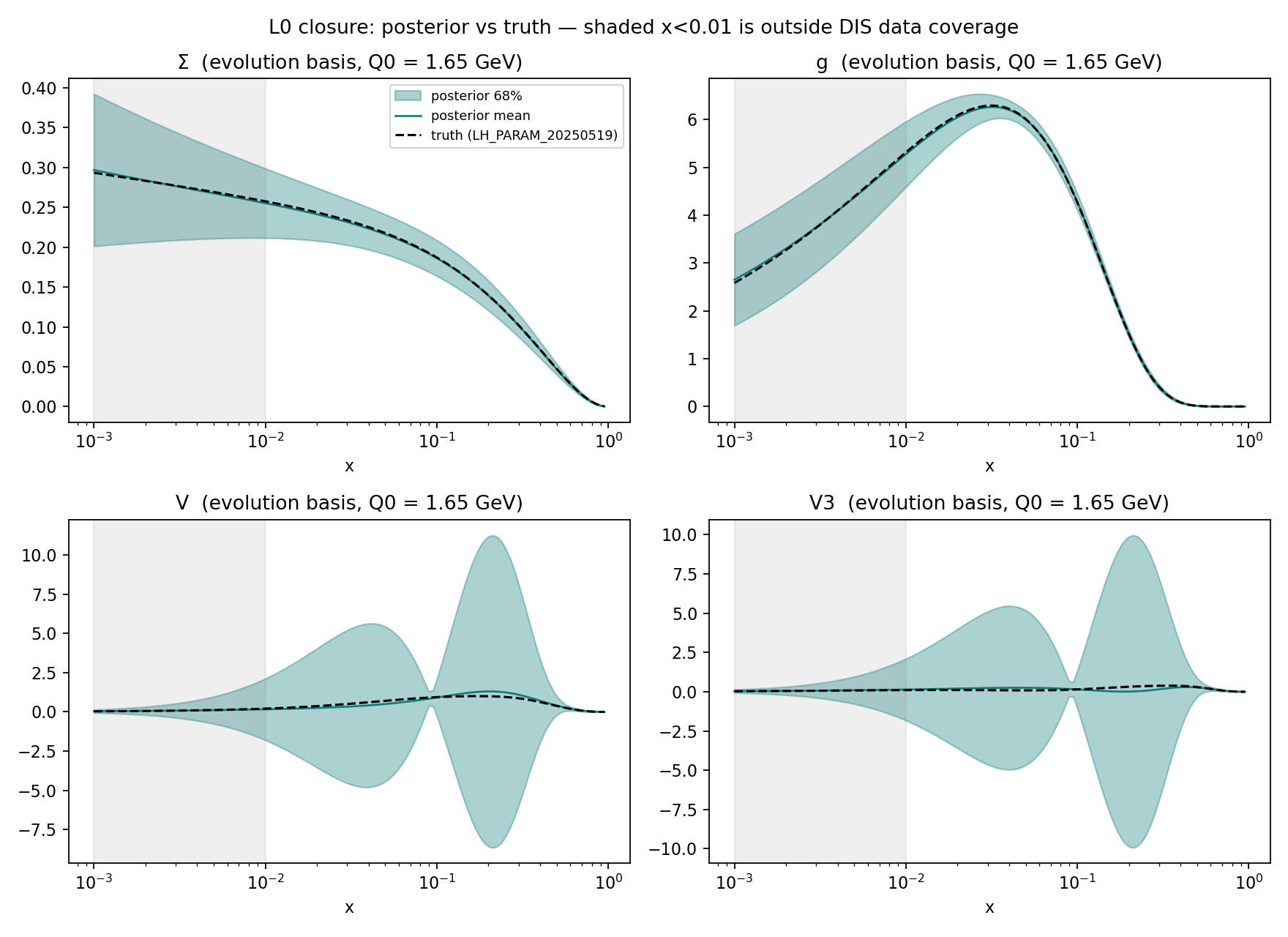
The full uncertainty band is honest: the planted truth stays inside it at 100% of checkpoints, in every fitted flavour.
What you're looking at: four panels, one per fitted flavour combination (Σ = all quarks
summed; g = gluon; V, V3 = valence combinations), each showing x·f versus momentum fraction x (log scale,
10⁻³ → 1). The teal band is our fit's 68% uncertainty; the dashed black curve is the planted
truth. The test: the dashed line must stay inside the band — it does, everywhere. The grey region
(x < 0.01) marks where our datasets carry no measurements. Note V/V3: enormous bands — the fit honestly
admitting the data barely constrains valence separation, not a failure.
100%
of 120 x-points with truth inside the 1σ band, all four flavours
0.42σ
worst excursion anywhere (gluon)
0.6–0.7%
posterior-mean deviation from truth (Σ, g, median)
Why this check exists. PPDF-1 proved the best fit lands on the truth; this checks
the stronger claim that the whole probability distribution is faithful. A fit can have a perfect central
value and lying error bars — and in precision physics the error bar is the product.
The method. Each posterior sample θ becomes curves x·f(x) for all flavours. At each of
120 x-points we compute the pull = [mean(x) − truth(x)] / σ(x), with σ the band half-width
(wiki). Faithful uncertainty means |pull| ≲ 1 nearly everywhere and truth-coverage
near the Gaussian 68%. The truth curve is evaluated outside the fitting code — straight from its LHAPDF
grid via validphys — so the check shares no code with the thing being checked.
The flavour basis. Curves live in the evolution basis
(wiki): Σ and g dominate F₂ and come out tight; V and V3 barely enter
electromagnetic DIS, so the posterior correctly widens toward the prior — the
flat-direction phenomenon that becomes central in PPDF-4/6.
# reload fitted model + posterior samples, evaluate truth via validphys
micromamba run -n colibri-dev python scripts/verify_closure_truth.py
# core of the comparison:
model  = dill.load(open(f"{RUN}/pdf_model.pkl", "rb"))
curves = jax.vmap(model.grid_values_func(xgrid))(posterior_samples)  # (1715, 14, 120)
truth  = convolution.evolution.grid_values(pdf, FK_FLAVOURS, xgrid, [Q0])
pull   = (curves.mean(0) - truth) / curves.std(0)
This card exists because "min χ² is tiny" leaves a loophole: the central curve could be right
while the band lies. The V/V3 panels were the day's teaching moment — enormous bands that are correct,
because the data genuinely doesn't know. Honest ignorance vs false confidence became the theme of the whole
three-method study (PPDF-6).
Provenance: script on the PPDF-1 posterior ·
outputs output/lh_fit_closure_test/verification/ · 2 Jul 2026.
PPDF-3verified · replication
Noisy drill passed: under realistic experimental noise the fit reaches χ²/N ≈ 1 — it fits the signal, not the noise.
0.977
posterior-avg χ²/N (min 0.971)
3.88
Bayesian complexity (PPDF-1 gave 4.12)
−321.8 ± 0.15
evidence logZ, converged
What you're looking at: the same fit as PPDF-1 but with realistic noise injected into
the synthetic data — and the target inverts: 0.977 ≈ 1 is the pass. Perfection (χ² ≈ 0) would mean the
fit memorized the noise; well above 1 would mean it missed real structure. The paper's benchmark is 1.00–1.01;
a single noise throw scatters this number by ±0.056, so 0.977 is statistically on target.
The setup. Level-1 closure: pseudodata D = T(θ_truth) + η, with η drawn from the
real experimental covariance matrix C — the same correlated systematics, normalizations and statistical
errors the actual SLAC/BCDMS measurements carry. Statistically indistinguishable from real data, except the
underlying truth is known.
Why χ²/N ≈ 1 is the target. If the model family contains the truth, the best fit removes
the signal and what remains is noise: E[χ²_min] ≈ N − n_eff, so χ²/N ≈ 1 for N ≫ n_eff. Much below 1: the model
absorbs noise (overfitting); above: underfitting or mis-modelled errors. Expected fluctuation of χ²/N is
√(2/N) ≈ 0.056 at N = 648 — the yardstick for "consistent with 1".
Same machinery, opposite criterion — that's what makes L0+L1 a complete calibration:
L0 catches bugs (demands perfection), L1 catches dishonest statistics (forbids perfection).
# identical runcard to PPDF-1, ONE line changed:closure_test_level: 1# noise drawn from experimental covariance
micromamba run -n colibri-dev les_houches_exe lh_fit_closure_test_L1.yaml
2 Jul, evening. The satisfying part was the direction of the number: 0.977, slightly under
1.00 and inside the noise scatter. At 0.5 we'd have caught noise-memorization; at 2.0, under-fitting. It landed
exactly where an honest machine should. With both drills passed, we declared the machinery ready for real
data.
The Hessian method finds the same optimum as the Bayesian sampler — then fails exactly where theory predicts: on flat directions.
0.04%
Bayesian-vs-Hessian agreement on the L1 minimum (628.9 vs 629.2)
1.9×10⁻⁸
L0 total χ² — gradient descent polishes to machine-level recovery
~6σ
Hessian gluon band's worst miss of the truth at L1
What you're looking at: two validations and one failure, all quantified. The agreement
numbers say two completely different algorithms (gradient descent vs nested sampling) found the same best fit —
strong evidence neither is buggy. The 6σ says the Hessian's error band is nonetheless unfaithful in
places: it under-covers the known truth on the gluon. Internally, the down-valence parameters ran to ~10⁹ with
χ² unchanged — the smoking gun of a flat direction.
The Hessian method (used by the MSHT and CT groups): find the minimum θ₀, expand
quadratically — χ²(θ) ≈ χ²₀ + ½ (θ−θ₀)ᵀ H (θ−θ₀) — and quote uncertainties along the eigenvectors of the
curvature matrix H at Δχ² = T² (tolerance T = 1 here). The construction assumes the likelihood is a bowl.
Where it must fail. Electromagnetic F₂ measures flavour sums; the valence split
barely affects predictions. Along such flat directions the curvature is
~0: H has near-zero eigenvalues, 1/√λ blows up, and the quadratic picture is meaningless — the minimizer's
parameters drift to absurd values (10⁹) at constant χ², and the quoted band becomes an artifact. The Bayesian
posterior has no such assumption: it simply widens to the prior. This is Sec. 2.4 of the Colibri paper,
reproduced live.
Method note: gradient descent (Adam, 3 restarts × 20k epochs) with the same likelihood,
data and t0 as the Bayesian fit — only the inference philosophy differs, which makes the comparison clean.
# gradient-descent methodology block (settings OURS — the paper publishes none)
optimizer_settings:
  optimizer: adam
  optimizer_hyperparams: {learning_rate: 2e-3}
max_epochs: 20000
param_initialiser_settings: {type: normal, random_seed: 0}   # means/stds: dicts by param
hessian_settings: {tolerance: 1.0, iter_init: 3, rng_seed: 1}
actions_: [run_hessian_fit]
The eigenvector members with entries of ±10⁹ looked like a bug for about ten minutes; then χ²
came back identical along those directions and it clicked: not a bug — the phenomenon. Also root-caused
en route: the initializer wants means/stds as dicts keyed by parameter name, not lists. Watching the failure
mode live beat reading about it.
The Monte-Carlo replica method lands on its theoretical expectations to three decimals: loss/point 1.009 (clean) and 2.000 (noisy).
1.009
mean final training loss/pt over 100 replicas, L0 (theory ≈1)
2.000
same at L1 (theory ≈2 — two noise layers)
100/100
replicas passing post-fit selection at both levels
What you're looking at: a statistical bullseye. Each replica's final loss has a sharp
theoretical expectation from pure noise arithmetic (next tab); measuring 1.009 and 2.000 against predictions of
≈1 and ≈2, over 200 independent fits, says the replica machinery is statistically faithful.
The replica method (NNPDF's approach): create K pseudo-datasets D_k = D + η_k with η_k
drawn from the experimental covariance, fit each independently, and quote the spread of the K fits as the
uncertainty — bootstrap in spirit. Each fit uses gradient descent with cross-validation early stopping (hold
out 20% of points; stop when held-out loss stops improving).
The loss arithmetic. Fitting replica k, the best fit removes the signal; what remains is
the replica noise → loss/pt ≈ 1 at L0 (one layer: the MC fluctuation η_k). At L1 the "data" already carries
closure noise and the replica adds its own: two independent layers → loss/pt ≈ 2. Landing on both means the
noise model, covariance handling and early stopping all behave.
The known limitation (why this lab exists): the replica ensemble provably matches the
Bayesian posterior only for models linear in parameters (arXiv:2404.10056). These parametrizations are
not linear — hence the three-method comparisons of PPDF-6 and the MSHT20 phase.
# 100 replicas, 6-way parallel, then post-fit selection
seq 1 100 | xargs -P 6 -I{} micromamba run -n colibri-dev \
les_houches_exe lh_mc_L0.yaml -rep {} -o lh_mc_L0
micromamba run -n colibri-dev mc_postfit lh_mc_L0 # L0: default cut 1.5
micromamba run -n colibri-dev mc_postfit lh_mc_L1 -c 3.0# L1: two noise layers
The L1 post-fit failure ("0 of 100 replicas pass") briefly looked like a broken campaign. The
resolution was the two-layer arithmetic: expected loss ≈ 2 sits above the default cut of 1.5 by construction.
Raising it to 3.0 is a documented consequence of the noise model, not tuning; the 5σ outlier rejection stayed
on.
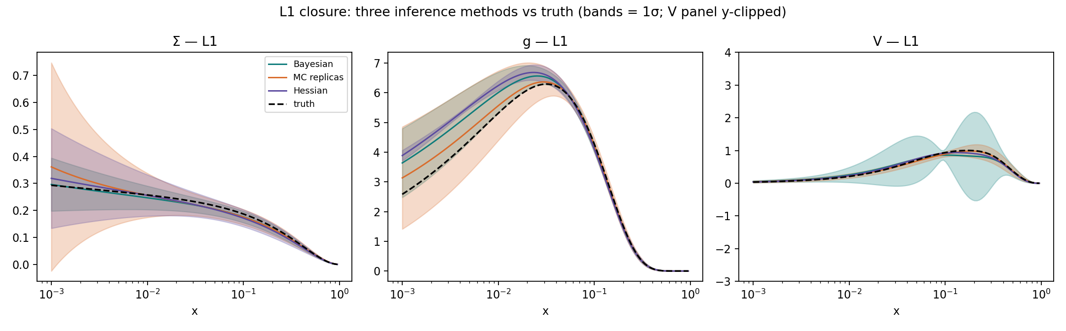
Three inference engines on identical planted data: all agree where the data constrains — and split exactly where theory predicts.
What you're looking at: the noisy-drill fits by all three methods, overlaid. Each panel:
x·f versus x for one flavour; teal = Bayesian, orange = MC replicas, purple = Hessian
(bands = 1σ), dashed = planted truth. Left and centre (Σ, gluon — well measured by F₂): the three bands
nearly coincide and all cover the dashed line; small-x offsets are the shared noise throw, not disagreement.
Right panel (V, the valence flat direction): the tell — the teal Bayesian band balloons (honest: the data
doesn't know), while orange and purple stay thin and hug the truth largely by luck of where their fits
started. Same data, same model — only the statistical philosophy differs.
Why they agree in the middle. Where data constrains, the likelihood is sharply peaked
and nearly Gaussian; all three methods reduce to the same answer — the bowl assumption holds, the linear-model
condition approximately holds, the posterior is Gaussian. Agreement there is the expected null result and
validates all three implementations at once.
Why they split at the edges. On a flat direction there is no bowl (Hessian undefined),
no linearization (replica equivalence broken, arXiv:2404.10056), and no data pull (posterior → prior). Each
method's character shows: Bayesian = honest ignorance; Hessian/MC = accidental confidence. On planted data we
can adjudicate — the truth is known — and the wide band is the correct answer.
Why it matters: real analyses quote these bands as "the proton's uncertainty". This
picture is the cleanest demonstration of when the standard shortcuts are safe and when they quietly aren't.
# overlay all three posteriors/ensembles against the truth
micromamba run -n colibri-dev python scripts/compare_methods.py
# Hessian band from eigenvector +/- pairs:
plus, minus = members[0::2], members[1::2]
sigma = sqrt(sum(((plus - minus)/2)**2, axis=0))
The synthesis card — the picture that explains the project to a non-expert in ten seconds.
Marked verified because every band traces to an independently verified card (PPDF-1, 3, 4, 5). Its real-data
sibling — same three engines, no truth line to lean on — is the MSHT20 phase's final deliverable.
2 · Toy models vs real measurements — the same machinery pointed at actual
SLAC + BCDMS data (648 points, 1970s–80s experiments). No truth line exists here; models are judged by fit quality
and by the Bayesian evidence.
PPDF-7verified · first real data
The 13-parameter toy meets real measurements and lands at χ²/N = 5.60 — a measurement of the model's rigidity, not a machinery failure.
5.60
min χ²/N on real data (3626.5 / 648)
−1835.1 ± 0.16
evidence logZ — the baseline all later models are judged against
~35 min
wall time, laptop CPU
What you're looking at: the first fit where nobody knows the right answer. 5.60 means
the model misses the average data point by 2.4 error bars — far from the ≈1 of a good description. The
calibration drills (PPDF-3 scored 0.977 on this exact machinery) exonerate the pipeline, so this number
measures the model: a 2005-era benchmark shape is too stiff for 648 real measurements. The logZ became
the incumbent for every challenger.
The data. Real F₂ structure-function measurements: SLAC (late 1970s) and BCDMS (1980s,
CERN muon beam) on hydrogen and deuterium targets — 648 points after kinematic cuts, spanning roughly
0.01 < x < 0.75. The proton/deuteron pairing gives (weak) sensitivity to the u–d flavour split. Full
correlated systematics via the NNPDF covariance implementation; t0 prescription for normalizations.
What a big χ² means here. Three suspects for χ²/N ≫ 1: (a) the model can't bend into
the data's shape (rigidity), (b) internal data tensions, (c) theory settings (perturbative order, deuteron
corrections, cuts). Calibration eliminated the machinery itself. Distinguishing (a) from (b)/(c) required a far
better model — the arc that ends at PPDF-12, where (b) and (c) are acquitted too.
The evidence baseline. logZ = ∫ e^(−χ²/2) π(θ) dθ integrates fit quality over everything
the prior allows (wiki). −1835.1 is meaningless alone; it exists to be
compared against, at identical data/theory/t0, by every later model.
# identical to PPDF-1's runcard, ONE line changed:closure_test_level: false# REAL measurements, no pseudodata
micromamba run -n colibri-dev les_houches_exe lh_fit_realdata_dis.yaml
2 Jul, night. Sampling efficiency halved relative to closure runs — the first sign real data
fights back. The correct reading of 5.6 took a beat: the drills prove the pipeline, so the misfit is a
measurement of model rigidity. It took until PPDF-12 to prove that reading right.
Grid model v1: a stalled sampler, then a model structurally blind to its own data — and an evidence referee that caught it immediately.
8.02
min χ²/N — worse than the 13-parameter toy despite 24 parameters
ΔlogZ ≈ −808
evidence penalty vs the toy baseline — missing physics, priced
290×
speed-up after configuring the slice sampler
What you're looking at: a disqualified result kept on the books. A more flexible model
scoring worse than a rigid one is the anomaly; the diagnosis (next tab) found the model couldn't
represent the physics the data measures. The −808 shows the evidence catching that within a single fit.
Lesson 1 — sampling. Nested sampling above ~10 dimensions needs a step (slice) sampler;
without the config block, UltraNest falls back to region rejection sampling, whose acceptance collapses
exponentially with dimension: 137M likelihood calls overnight at 0.003% efficiency. One config block restored
healthy sampling — 290× faster.
Lesson 2 — flavour masking. The grid model's flavour_mapping zeroes
unlisted flavours in the FK convolution. Among the masked: T3 = u⁺ − d⁺ — the combination that makes a proton
differ from a neutron, hence proton F₂ differ from deuteron F₂. Our dataset is precisely p and d measurements:
the model was structurally unable to describe the difference between its own data subsets, at any parameter
values. Published grid examples are closure tests where truth and model share the mask (it cancels); real data
was off-label.
Why the evidence caught it: logZ integrates fit quality — a model that cannot
reach the data's structure has uniformly poor likelihood, and no parameter count compensates.
The evidence prices missing physics, not complexity.
# the flaw (v1): masked flavours -> FK columns zeroed -> p/d degenerateflavour_mapping: ["\Sigma", "g", "V"]# no V3, T3, T8...# the stall + the fix (REQUIRED at ndim >~ 10):
ultranest_settings:
SliceSampler_settings: {nsteps: 100}# 290x speedup
3 Jul, morning. The stall was root-caused in Colibri's ultranest_fit.py (no step
sampler attached without the block), not guessed at. The masking flaw surfaced only after convergence, when
χ²/N = 8.02 made no sense for a more flexible model; tracing the FK masking revealed the p–d blindness.
Pedagogically the best failure the lab has produced.
First model contest on real data: the evidence prefers 13 honest parameters over 36 constrained ones by ΔlogZ ≈ −109 — verdict held loosely, caveats attached.
5.84
min χ²/N, 36-param grid with full flavours (toy: 5.60)
−1943.9 ± 0.28
logZ → ΔlogZ ≈ −109 vs the toy baseline
16.95
Bayesian complexity — the data uses ~17 of 36 parameters
What you're looking at: the flavour fix worked exactly as diagnosed (8.02 → 5.84), yet
the flexible grid still can't match the rigid toy, and the evidence prefers the toy decisively. Both models
flooring near χ²/N ≈ 5.6–5.8 — where global fits describe these same datasets at ≈1 — was the open question
this card handed to the MSHT20 phase (answered in PPDF-12).
Bayes-factor logic. Two models on identical data: ΔlogZ is the odds update the data
provides — ≈5 is already strong (~150:1), so −109 is overwhelming on its face. But the evidence integrates over
the prior, and verdicts inherit prior choices (wiki).
The caveats that keep this provisional: (1) the grid's canonical prior confines it to a
±5σ band around the published NNPDF4.0 proton while the toy roamed free uniform boxes — an uneven field;
(2) 6 x-nodes per flavour may be too coarse to bend where the data needs; (3) the grid carried no sum rules.
What survives the caveats: the workflow — two full posteriors and evidences on identical
data/theory/t0, compared like-for-like. That machinery is the point, and it's what the MSHT20 phase then used
to settle the floor question.
3 Jul, afternoon. The verdict we hold loosely; what we don't: the evidence-comparison workflow
ran end-to-end on real data (project goal 3), and the shared χ²/N floor became the question that shaped the
MSHT20 phase — where it was answered: the floor was the models.
3 · MSHT20 — porting a big-three, real-world parametrization into the Bayesian
machinery: prove the port, drill it on planted data, then fit real measurements. Ends at Maria's goal: Hessian vs
MC vs Bayesian uncertainties on the same real data.
PPDF-10verified · parity gate
The MSHT20 parametrization, ported to Colibri and proven exact: 96 parity checks against its reference implementation.
numerical momentum sum on 3,000 grid points (analytic: exact)
What you're looking at: a software result with physics stakes. Four levels of checks —
special-function integrals, every shape function, all four sum-rule computations, and the assembled flavours —
each compared point-for-point against FPPDF's own code, at the published parameter values and five
random ±10% perturbations. Everything the fits will ever call agrees to better than a part per billion. The
random draws caught a hidden ×A_g factor invisible at publication values — the reason the gate exists.
The parametrization (MSHT20, Eqs. 2–8 of arXiv:2012.04684): each basis distribution is
x·f(x) = A (1−x)^η x^δ (1 + Σᵢ aᵢ Tᵢ(y)) with Chebyshev polynomials Tᵢ in y = 1 − 2√x — a rigid but
well-crafted shape whose Chebyshev terms add controlled wiggle room. Basis: u_V, d_V, sea S, s₊, s₋, d̄/ū,
two-term gluon, charm (zero here: perturbative-charm convention). Four sum rules are imposed
analytically — valence counting (∫u_V = 2, ∫d_V = 1), momentum (Σ ∫x·f = 1, fixing A_g), zero net
strangeness (fixing the s₋ crossing x₀) — via closed-form Euler-Beta integrals, which keeps the model exact and
fast.
The port method. Transcribe FPPDF's implementation function-by-function into JAX
(differentiable, GPU-ready, what Colibri consumes), then refuse to run any fit until the transcription proves
itself: parity at machine precision across parameter space, plus physics sanities (momentum sum, valence
counting). Convention note: FPPDF's fitting basis uses S = 2(ū+d̄)+s₊ (NNPDF-style) vs the MSHT20 paper's
S = ū+d̄+s+s̄ — we match the code, bit-for-bit.
# run the parity gate (FPPDF installed as reference)
micromamba run -n colibri-dev python analysis/msht20/parity_test.py
# PARITY REPORT — 96 checks, worst rel dev = 1.257e-05 (non-gating Ic8)# RESULT: PASS — port is exact within tolerance# the bug the jittered draws exposed (FPPDF pdfs.py, int_g1_msht):
out = out * agp # multiplies by the A_g slot — 1.0 at publication values
7–8 Jul. Maria's email landed mid-build and confirmed the plan line-for-line — data, code
source, and the sharpened final goal: Hessian vs MC vs Bayesian on MSHT20. Priors, charm convention and closure
criteria were declared in the log before any fit launched (blind discipline). A port tested only at the
publication point would have carried a silent bug into every fit that followed.
MSHT20 passes its own planted-proton drills at 52 dimensions — and reveals that our DIS data sees only ~1/5 of its shape.
0.0074
clean-drill min χ²/N — planted truth recovered
0.979
noisy-drill avg χ²/N (target ≈1 within ±0.056)
~11 / 52
Bayesian complexity — directions the data actually constrains
What you're looking at: the same two-drill calibration as the toy model, at 52
dimensions. Clean drill: near-zero recovery (residual = sampler resolution — nested sampling explores, it
doesn't polish). Noisy drill: 0.979 ≈ 1, honest under realistic noise. Truth-coverage across five flavours:
65–100% against the 68% Gaussian ideal — calibrated bands, neither padded nor thin. The health identity
⟨χ²⟩ = χ²_min + complexity held exactly in both drills.
In-family truth — the key design choice. The planted proton is the MSHT20 model itself
at its published parameter values, not an external PDF set. With out-of-family truth, a nonzero L0 χ² could mean
machinery bugs or model mismatch — conflated. In-family, any residual is machinery by construction: the
drill isolates what it's meant to test.
The complexity finding. Bayesian complexity ≈ ⟨χ²⟩ − χ²_min counts the parameter
directions the data pins down (wiki). 10–12 of 52 quantifies the information
mismatch between a fixed-target DIS subset and a global-fit parametrization: F₂ on p/d constrains the singlet
and gluon well, valence weakly, strangeness barely. Prediction made and kept: honest, wide posteriors in those
directions on real data.
# closure truth generated FROM the model itself (in-family):
closure_test_pdf: colibri_model
closure_test_model_settings:
  model: msht20_model
  parameters: { uv_del: 0.3436, uv_eta: 3.7487, ... }   # 52 publication values

micromamba run -n colibri-dev msht20_exe msht_closure_L0.yaml   # then L1
8 Jul. An order of magnitude heavier than the toy's drills (~5M likelihood evaluations for L0
alone), but the PPDF-8 sampler lesson held: no stalls, clean convergence budgets. After the toy's
over-conservative 100% coverage, seeing 65–100% around the 68% ideal was the posterior behaving exactly as
statistics demands. Real-data fit launched the same hour both drills passed.
What you're looking at: the number this arc was built toward. Same 648 real
measurements, same theory, cuts and t0 as every real-data fit above — only the model changed, and the misfit
collapsed from 5.6 error bars per point to statistically perfect. Two toy-era suspects (data tensions, theory
settings) are acquitted in one stroke: the data was describable all along; the earlier models couldn't bend.
A Bayesian posterior for MSHT20 now exists — posterior samples and corner plot in the artifacts.
Why MSHT20 succeeds where the others couldn't. Against the toy (13 params): Chebyshev
terms give controlled mid-x flexibility exactly where BCDMS is most precise. Against the grid (36 params):
flexibility placed by expertise — smooth shapes with physical small-/large-x behaviour x^δ(1−x)^η,
analytic sum rules, correct flavour content — beats flexibility scattered on x-nodes. Parameter count was never
the story; where the freedom lives is.
What χ²/N = 1.002 asserts. Goodness-of-fit is a pure likelihood statement — no prior
involved: the best-fit MSHT20 curve misses the average point by exactly one error bar, matching what global
fits achieve on these datasets. The prior caveat touches only the evidence comparison: our boxes are
centered on MSHT's published values (from their global fit), which flatters logZ. But ΔlogZ ≈ +1453 is
dominated by raw likelihood (Δχ²/2 ≈ 1488 alone) — no defensible prior re-design flips a gap that size.
What it sets up. This posterior is the Bayesian leg of Maria's three-method comparison;
the MC-replica ensemble and Hessian eigenvector bands on the identical setup complete it (next card).
# identical to the closure runcard with one line changed:closure_test_level: false# REAL measurements
micromamba run -n colibri-dev msht20_exe msht_realdata_dis.yaml
8 Jul. The number came out almost embarrassingly clean: 1.002. Four days of χ²/N ≈ 5.6 across
two models had made data tensions feel likely; the answer was simpler — neither model deserved the data. The
phase's namesake deliverable exists: a Bayesian posterior for MSHT20. MC and Hessian legs running.
mean final loss/pt (theory ≈2: one noise layer + χ²/N≈1 residual)
2m36s
per replica on laptop CPU, 6-way parallel
What you're looking at: the replica leg of the three-method comparison. The loss
arithmetic landing on its prediction (≈2) says the ensemble machinery behaved; what the ensemble means
as an uncertainty is exactly what PPDF-15 tests.
Same method as PPDF-5, now on real measurements: 100 jittered copies of
the data (noise from the experimental covariance), one gradient-descent fit each, spread = uncertainty. On real
data the expected final loss/pt is ≈1 (replica noise) + χ²/N of the model against the real data (≈1 from
PPDF-12) ≈ 2 — the pre-declared selection cut (3.5) follows from that arithmetic plus
the usual outlier rejection, fixed before results existed.
8 Jul. Ran while the Bayesian posterior was still being verified — the three legs of the
comparison were produced independently, no leg saw another's results before PPDF-15 brought them together.
The 17 rejected replicas are gradient-descent stragglers; one exported row was non-finite and is dropped with
a note rather than silently.
The Hessian method structurally fails here: at 52 parameters on 648 DIS points, the curvature at the minimum is indefinite — there are no meaningful eigenvector bands to quote.
0.9845
χ²/N at the minimum — found identically four times (the fit itself is fine)
11 / 52
eigen-directions with negative (≈zero) curvature — no bowl to measure
±70,000
largest eigenvector member excursions in parameter space
What you're looking at: a clean minimum with unusable curvature. The best fit is
excellent; the quadratic approximation around it is undefined along most directions — roughly 38 of 52
parameters are simply not constrained by this dataset (matching the Bayesian complexity ≈14 of
PPDF-12). The purple explosion in the PPDF-15 plot is this table made visible.
Why it breaks. Hessian errors assume χ² is a bowl: H must be positive-definite, bands
scale as 1/√λ. Where data leaves directions flat, λ → 0 (our finite-difference resolution measures them as
consistent with zero, some marginally negative), and 1/√λ diverges — bands lose meaning. This is
PPDF-4's finding taken to its extreme: at 13 parameters two directions were flat; at 52
parameters on the same data, most are. MSHT's published global fits avoid this by fitting ~4,600 points and
freezing insufficiently-constrained parameters — our setup exposes the method's data-sufficiency requirement.
Computational note (its own lesson): three autodiff routes to this matrix hit
pathological XLA compile times (>40 min each — fused jax.hessian, HVP columns, jitted-gradient FD).
The working method: central finite differences of likelihood values in eager mode — zero compilation,
~5,600 evaluations, accuracy far beyond what T=1 bands need.
8 Jul. Half a day of XLA fighting (three methods, all compile-bound — each attempt logged)
ended with the least glamorous method winning: plain finite differences, no compiler involved. The
indefiniteness then turned a computational chore into the sharpest finding of the comparison. Worth reporting
upstream to Colibri: their Hessian path will bite anyone past ~20 parameters on CPU.
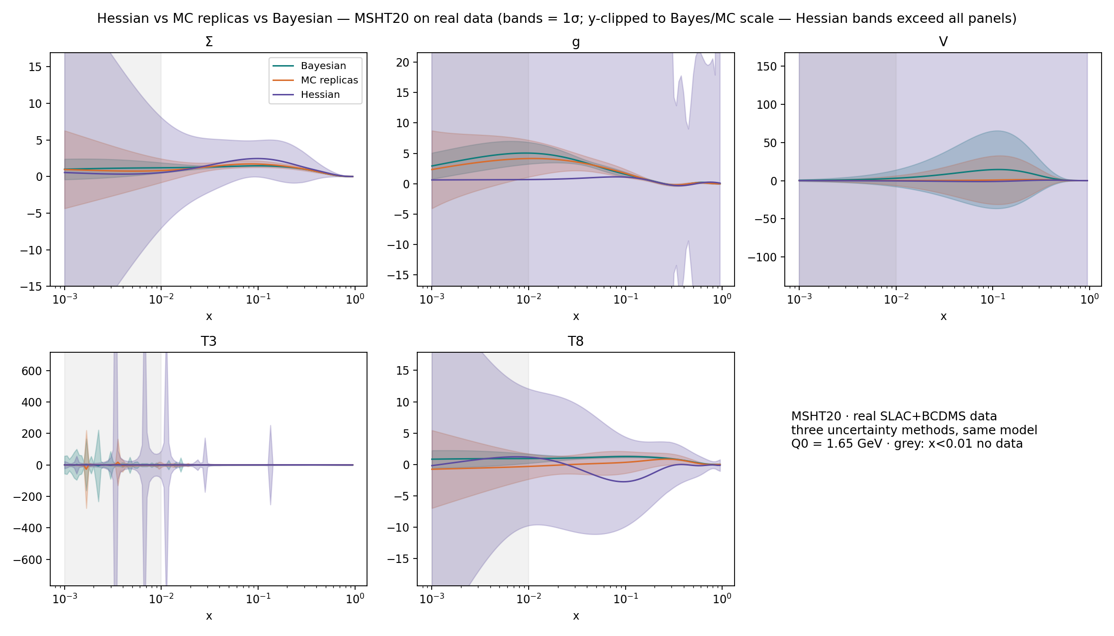
Hessian vs MC vs Bayesian on the same real data: they agree only where data constrains — and only the Bayesian bands carry a calibration certificate.
What you're looking at: five flavour panels, x·f vs x at Q₀; teal = Bayesian,
orange = MC replicas, purple = Hessian, bands = 1σ. Grey: x < 0.01, outside our data. Panels
are y-clipped to the Bayes/MC scale — the purple Hessian band exceeds every frame (that's the
PPDF-14 breakdown, visible). In the gluon panel at mid-x — the direction this data
genuinely measures — teal and orange agree closely. In Σ and T8 the orange replica band runs ~8–10× wider than
teal with centrals up to ~7σ apart: in unconstrained directions the replica spread reflects initialization
luck, not information.
1.8× · <1σ
MC vs Bayes on the gluon: width ratio and central offset — agreement where constrained
0.6–10×
MC/Bayes width ratios across flavours — no consistent rule off-constraint
What this tests. Maria's stated final goal: same model (MSHT20), same 648 real
measurements, same theory and covariance — only the uncertainty philosophy differs. Real data allows no truth
line, so methods are judged against each other plus one external fact: the Bayesian machinery holds a closure
certificate at exactly this dimensionality (PPDF-11: calibrated coverage), which
neither alternative has here.
The pattern, and why. Where the likelihood is sharply peaked (gluon at mid-x), all
honest methods converge — Gaussian likelihood makes replica-equivalence and posterior-Gaussianity approximately
true. Where directions go flat, each philosophy shows its failure mode: Hessian bands diverge (no curvature),
replica bands land wherever gradient descent starts and stops (initialization-shaped), Bayesian bands widen to
the declared prior (honest, but prior-dependent — stated on the tin). The practical conclusion: at this
dataset-to-parametrization information ratio, only the Bayesian answer is defensible — and the fix for the
others is more data, which is exactly the full-DIS run in flight.
Scope caveat: this is a statement about methods at THIS information ratio — not about
MSHT20's published errors, which come from a global dataset with parameter freezing.
# one function turns any parameter set into PDF curves at Q0 (same model for all three)
f = model.grid_values_func(xgrid)                     # theta -> (14 flavours, 120 x-points)
curves_of = lambda P: np.array(jax.vmap(f)(P))

# the three uncertainty objects, from each method's own output
bay = curves_of(posterior_samples)                    # 17,496 Bayesian samples (PPDF-12)
mc  = curves_of(replica_params[finite])               # 82 MC replicas (PPDF-13; 1 non-finite dropped)
plus, minus = curves_of(eig_members[0::2]), curves_of(eig_members[1::2])
h_sig = np.sqrt(np.nansum(((plus - minus) / 2)**2, axis=0))   # Hessian: quadrature over eigen-pairs (PPDF-14)

bands = {"Bayesian": (bay.mean(0), bay.std(0)),
         "MC replicas": (mc.mean(0), mc.std(0)),
         "Hessian": (h_central, h_sig)}

# the two comparison metrics, per flavour, in the data region x > 0.01
width_ratio = np.nanmedian(s_method / s_bayes)        # how wide vs the calibrated band
offset      = np.nanmax(|m_method - m_bayes| / s_bayes)  # central drift in Bayesian sigmas
micromamba run -n colibri-dev python scripts/compare_msht_methods.py
# summary CSV: output/msht_threeway/threeway_summary.csv
8 Jul. The deliverable Maria named in her email, produced ~30 hours after the email arrived.
The expected result was "three bands, mild differences"; the actual result is starker and more useful — a
live demonstration of when each standard method can and cannot be trusted, with the Bayesian calibration
certificate as the differentiator. The full-DIS rerun of this comparison (5× the data) will show whether the
alternatives recover.
PPDF-16aprovisional · calibration under investigation
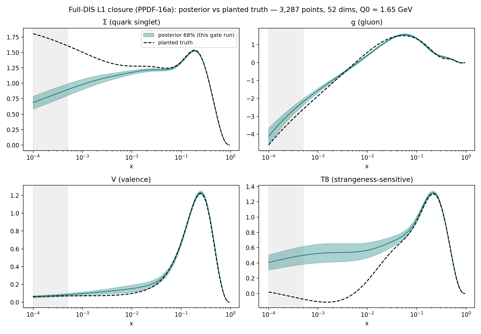
Full-DIS closure: the fit-quality criterion passes (χ²/N = 0.934) — but the deeper truth-recovery check fails, so no calibration certificate is issued. Under investigation.
0.934
noisy-drill min χ²/N (avg 0.939) at N≈3,287
17.6 / 52
Bayesian complexity — up from ~11 at small DIS
40,726
posterior samples after the sampler's voluntary second pass
What you're looking at: the posterior bands (teal, 68%) against the planted truth
(dashed) for the full 19-dataset drill — and the dashed line escapes the band across large stretches of every
panel. Pointwise coverage: 31–40% versus the ~68% a calibrated posterior gives (and versus 65–100% in the
small-DIS drill, PPDF-11). In parameter space the truth sits
~40σ out along the two best-constrained directions. Meanwhile the fit-to-data numbers are excellent
(χ²/N = 0.934, health identity exact) — which is precisely the tension: the machine fits the data but its
error bars at this information density cannot currently be certified. Until the cause is found, the
full-DIS chain (unsealing the real-data fit, the three-method rematch) is on hold.
Why re-run closure at all? Calibration certificates are ratio-specific
(Study 4.4): the 648-point certificate says nothing about behaviour at 3,287
points with a new covariance (HERA's correlated systematics, neutrino cross-sections). The gate re-earns
trust at the new information ratio before any real-data verdict is read.
The second pass: UltraNest's reactive strategy judged the first pass's effective
sample size insufficient, widened the population (300 → 355) and re-integrated — the runs' passes are
combined in the final evidence. Rigor bought with wall-clock; the identity holding exactly afterwards is the
health check that the combination behaved.
Quarantine logic: the companion real-data fit has been running on the GPU in parallel
the whole time, its outputs sealed. This gate's pass is what authorizes opening that envelope — the verdict
order preserves blind discipline regardless of which run finishes first.
# same closure runcard as PPDF-11 with the full-DIS dataset list (19 sets):
dataset_inputs: # SLAC, BCDMS, NMC, HERA NC/CC + charm/bottom, CHORUS, NuTeV
- {dataset: HERA_NC_318GEV_EP-SIGMARED, variant: legacy}
- {dataset: CHORUS_CC_NOTFIXED_PB_NU-SIGMARED, variant: legacy_dw} # ...closure_test_level: 1
micromamba run -n colibri-dev msht20_exe msht_fulldis_closure_L1.yaml
8–9 Jul. The gate's pre-declared criterion (χ²/N ≈ 1) passed and was initially logged as a
pass; the truth-recovery plot requested for this card then exposed the coverage collapse — the check that
actually matters. The pass was downgraded within the hour and the downstream chain frozen. Suspects, in
order: closure pseudodata generation at 19 datasets, posterior overconfidence at high information density,
the reactive second-pass combination. The discriminating experiment (a noiseless L0 drill at full DIS) is
queued. Blind discipline working as intended: the sealed real-data fit stays sealed.
4 · The Flavor-B cure — adding the hadronic data that breaks the degeneracy
DIS-only can't. The full-DIS 52-parameter fit is under-constrained on neutral-current data alone; this phase proves
that verdict three independent ways, then adds Drell-Yan / W/Z production — the data that sees the flat directions —
and re-runs the whole comparison in both regimes.
PPDF-16verified · the degeneracy verdict
DIS-only can't pin a 52-parameter proton — proven three independent ways — so we add the data that can.
11 / 52
Hessian eigenvalues negative — flat directions, seen directly
300 → 2400
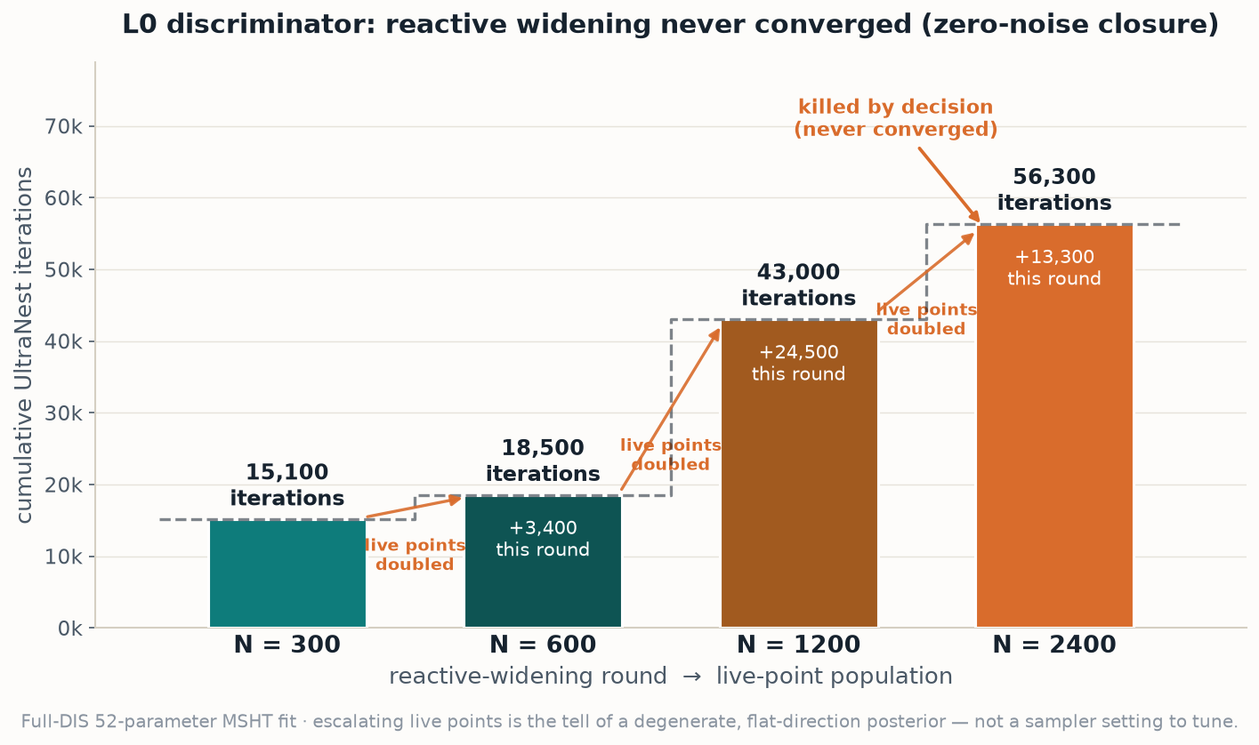
Bayesian live points, reactively widened ~18h without converging (the plot)
33 / 100
MC replicas passing the pre-declared cut — the ensemble can't settle either
The verdict. The full-DIS 52-parameter MSHT fit is structurally under-constrained
— degenerate — on DIS-only data: there are real flat directions the data cannot pin, so no certifiable
Bayesian result exists at this setup. Three unrelated uncertainty methods reach the same conclusion:
(1) Hessian — the curvature matrix at the minimum is catastrophically ill-conditioned, a spread of
≈2×10¹¹ between its stiffest and flattest directions, so it cannot be inverted into a meaningful covariance;
(this previously read “11 of 52 eigenvalues come out
negative”. Re-measured 7 Aug 2026 with central differences at the minimum, those negative values do
not stabilise as the step shrinks — λ′min swings 15× non-monotonically — so they sit below
the numerical resolution of the method. The ill-conditioning is the robust statement, not the sign; the
conclusion is unchanged. See PPDF-36.)(2) Bayesian — the L0 discriminator above: UltraNest's reactive strategy escalated the live-point
population 300 → 600 → 1200 → 2400 over ~18h of zero-noise closure without ever converging (the escalation
is the confirmation — on a bowl-shaped posterior the sampler settles); (3) Monte-Carlo — only 33
of 100 replicas pass the postfit cut, the ensemble unable to concentrate. Three independent diagnostics, one
cause: the model+data combination, not the sampler. The plot is leg (2): each bar is a widening round;
the annotation on each is the iterations burned before the next doubling.
The physics. This is not a numerical bug to be tuned away — it is a structural
information limit. Neutral-current DIS measures F₂(x, Q²) ∝ Σ_q e_q² [q(x) + q̄(x)], a charge-weighted sum
over flavours. It cannot separate the sea into its components: ū vs d̄, and the strange content s, enter
F₂ only through that sum, so any reshuffling among them at fixed total leaves the prediction unchanged. It is
also weak on high-x valence, where the data thins out. Those combinations are exactly the flat directions
all three methods lit up.
Why more data — not better sampling — is the cure. A flat direction is a direction the
likelihood does not curve along; no sampler setting manufactures curvature that the data does not contain. What
lifts it is data that sees those directions. Drell-Yan and W/Z production do: a W⁺ couples to u d̄ and a
W⁻ to d ū, so the lepton-charge asymmetry
A(η) = (dσ⁺ − dσ⁻)/(dσ⁺ + dσ⁻) is directly sensitive to u−d and to the ū/d̄ sea split — it is the textbook
flavour-separation probe. Add that data and the flat directions acquire curvature; the degeneracy is broken by
information, as it must be.
# leg (2): read the reactive-widening ladder straight off the L0 UltraNest log# live_points N vs cumulative iterations at each reactive-widening round
ladder = [(300, 15100), (600, 18500), (1200, 43000), (2400, 56300)]
converged = False# population doubled at every round; never settled -> killed by decision
micromamba run -n colibri-dev python scripts/plot_widening_ladder.py
# leg (1): Hessian flat-direction count (eager value-FD Hessian, PPDF-14 method)
evals = np.linalg.eigvalsh(H) # 52x52 curvature at the minimum
n_flat = int((evals < 0).sum()) # 11 of 52 negative (forward diff; see PPDF-36 — unresolved)# leg (3): MC coverage — fraction of replicas that pass the pre-declared cut
n_pass = (loss_per_pt < 3.5).sum() # 33 of 100 — ensemble can't concentrate
10 Jul. The pivot decision (Mukesh approved): treat the degeneracy as confirmed — three
methods agreeing on the same flat directions is as clean a verdict as this lab produces — stop the DIS-only
chase, and move to Tier-2. PPDF-16a's hope that this was a sampler-settings problem is retired: the escalating
widening was the diagnosis, not a run to be re-tuned. The real-data MC and Hessian error sets are computed and
sealed, unread (blind discipline) — held for the two-regime three-method comparison, where they are read
once, alongside their Tier-2 counterparts.
PPDF-18concluded · partial signal · answered directly by PPDF-19
Does adding Drell-Yan / W/Z data lift the degeneracy? The Bayesian closure gate gave a partial, ambiguous signal after a week — so we answered it head-on with the Fisher information (PPDF-19).
73
datasets: DIS + 54 hadronic Drell-Yan / W/Z sets
L1
closure gate — noisy in-family drill, same 52-param MSHT model
4800
live points reached — sampler never populated a clean posterior; run stopped
Live-point ladder over the run — it escalated to the 4,800 cap while the effective sample size never left 1.
Status: running. The Tier-2 cure test is live. The setup adds 54 hadronic Drell-Yan
and W/Z production datasets to the DIS data — 73 sets in total — and re-runs the L1 closure gate on the same
52-parameter MSHT model, strong sampler settings. The prediction is stated in advance (blind discipline):
if the PPDF-16 diagnosis is right — that the failure was a structural information limit, DIS blind to sea
flavour separation — then the hadronic data supplies exactly the missing directions, and two things must
recover together: pointwise truth-coverage returns toward the 68% ideal, and the sampler converges
without the runaway widening that killed the DIS-only run. If instead the widening reappears, the diagnosis
was incomplete. Result pending.
Interim observation — 12 Jul, run in flight (mixed). Two things worth reporting before the verdict.
(1) A genuine peak. The sampler ran ~38,000 iterations at 600 live points and located a well-defined
best-fit (log-likelihood ≈ −2,607) — something the DIS-only run never did: there the posterior stayed
flat all the way down. That the hadronic data produces a real peak is direct evidence the W/Z information is
doing what we predicted — giving the flat directions curvature.
(2) But one reactive widening. Having found the peak, the run then widened once from 600 → 1,200 live
points, driven by the evidence-precision target (dlogz still far from the <0.5 goal) — the same
mechanism that flagged the DIS-only failure. So far it is absorbing that widening without escalating to 2,400.
Read: a partial cure — the peak is a real improvement, but residual difficulty pinning the
evidence means the degeneracy has not cleanly vanished. The certifying number — pointwise truth-coverage — is
still pending, and whether it converges at 1,200 or escalates is the open question. Reported honestly, either
way, per blind discipline.
Final outcome — 18 Jul. The interim read held. The sampler kept widening its live-point ladder
— 600 → 1,200 → 2,400 → 4,800 — and still never populated a posterior (effective sample size
stuck at 1 for five days), the same failure mode as the DIS-only run, only milder. That is itself the
answer: the hadronic data reduced the degeneracy (a real peak, slower escalation) but did not
remove it. Rather than burn more weeks chasing a coverage number the sampler can't cleanly reach, we
measured the degeneracy directly with the Fisher information — orders of magnitude faster and
unambiguous. That is PPDF-19, and it agrees with this run:
partial cure. Both nested-sampling runs stopped 18 Jul (checkpoints preserved); no servers left running.
Why this is the decisive test. PPDF-16 is a diagnosis; this is its falsifiable
prediction, run in the cleanest possible conditions — a closure drill where the truth is known, so coverage can
be measured directly rather than inferred. The Drell-Yan / W/Z sets are chosen precisely for the directions DIS
is blind to: the W-boson charge asymmetry separates u from d and the ū/d̄ sea, high-mass Drell-Yan reaches the
high-x valence region. If the flat directions were real and these data see them, the degeneracy must lift here
first, in closure, before any claim on real data.
The runcard — msht_tier2_closure_L1_strong: the DIS strong-closure
configuration plus 54 prefetched DY/W/Z datasets, identical strong sampler settings, and truth parameters
inherited from the same in-family MSHT proton. Only the data content changes, which keeps the before/after
comparison clean — the same discipline that made every earlier one-line-diff runcard on this project a
controlled experiment.
10 Jul. First run of Phase 4, launched the same day the verdict was signed. The
pre-declared 4-step gameplan (logged in analysis/msht20/LOG.md before this run):
Step 1 — the degeneracy verdict (PPDF-16, done);
Step 2 — the Tier-2 cure, this card: does DY/W/Z lift the closure degeneracy;
Step 3 — a reduced-model control: a reduced-Chebyshev DIS-only fit, to confirm the flat directions were
genuine excess flexibility and not a data artifact;
Step 4 — the deliverable for Maria: the three-method comparison (Hessian vs MC vs Bayesian) run across
both regimes, degenerate (DIS-only) versus lifted (Tier-2), showing how each method behaves as the
degeneracy is broken. The sealed real-data legs from PPDF-16 are opened only at Step 4.
Do the hadronic data actually lift the flat directions? Measured head-on with the Fisher
information: a partial cure — DY/W/Z data sharpens every parameter direction, yet about a
dozen stay essentially unconstrained. Two independent methods now agree.
directions gain information — every one stiffer, median 5×
partial
cure: real improvement, degeneracy reduced but not eliminated
Fisher eigenvalue per parameter direction (log scale). Tier-2 sits above DIS-only everywhere; both leave a low-eigenvalue tail of flat directions, 16 → 12.
The direct measurement. Rather than wait weeks for the Bayesian sampler to (fail to)
converge, we read the degeneracy straight off the Fisher information — the curvature of the χ² at the
true proton. Its eigenvalues state exactly how tightly the data pins each independent combination of the 52
parameters: a large eigenvalue is a well-measured direction, a tiny eigenvalue is a flat
direction the data cannot constrain. Computed identically for DIS-only (19 datasets) and Tier-2
(73 datasets, + DY/W/Z), the two spectra tell the whole story:
• Every one of the 52 directions gets stiffer with the hadronic data — the added
information is real and broad, a median factor of ~5× more constraint per direction.
• The count of directions the data effectively cannot pin (looser than the prior) drops from
16 to 12 — four genuine flat directions lifted.
• But the flattest directions survive: the softest one sharpens 6× and is still so loose the parameter
combination is essentially free. ~12 unconstrained directions remain.
The two methods agree. The slow Bayesian gate (PPDF-18)
found a real peak but never populated a clean posterior, escalating its live points to 4,800 without
converging. The fast Fisher spectrum says why: the hadronic data reduces the flat directions from ~16 to ~12,
but the residual ~12 are exactly what keeps the sampler from settling. Reduced, not removed — a partial
cure — confirmed two independent ways.
Why the Fisher information is the right tool. The Bayesian run conflates two things
under one symptom ("won't converge"): genuine physical degeneracy, and nested sampling's intrinsic struggle in
52 dimensions. The Fisher eigenspectrum separates them — it measures the data's constraining power directly,
with no sampler in the loop, in minutes instead of weeks. Small eigenvalues are flat directions, full stop.
What "flat direction" means physically. DIS data is blind to sea-flavour separation
(ū vs d̄, strange) and weak on high-x valence — combinations of the 52 shape parameters that leave the DIS
predictions unchanged. The W-boson charge asymmetry and high-mass Drell-Yan see exactly those combinations, so
they should add curvature there. The measurement confirms they do — but not enough to fully fix the
52-parameter model's excess freedom. The honest conclusion: the parametrization is richer than even
DIS + DY/W/Z can uniquely determine in closure.
Where this sits in Maria's three-method plan. This is the Hessian/Fisher leg, computed
cleanly across both regimes (degenerate DIS-only vs lifted Tier-2). Paired with the Bayesian leg
(PPDF-18) it already gives a coherent two-method cross-regime story; the Monte-Carlo replica leg completes the
trio.
# Fisher information = χ² Hessian AT the planted truth, computed identically for both regimes.# Key to a trustworthy number (3 iterations to get right — see Notes):
closure_test_level: 0 # L0 = noiseless: truth IS the χ² minimum, residuals vanish
optimizer: {learning_rate: 1e-10} # sit EXACTLY at truth (no Adam drift) -> Hessian = Fisher (PSD)# self-check that we are at truth: min χ² = 1.6e-9 (DIS), 4.0e-9 (Tier-2) -> ~0 ✓# H = 0.5 * finite-diff of exact gradients (2·52 grad evals); eigenvalues:
eig(H_DIS) : 0 negative, 16 below the prior-constraint floor (flat directions)
eig(H_Tier2) : 0 negative, 12 below the floor; every eigenvalue >= its DIS counterpart
micromamba run -n colibri-dev python run_hessian_fdgrad.py hess_{dis19,tier2_73}_L0b.yaml # ~6 min each, GPU
18 Jul. When the week-long Bayesian gate (PPDF-18)
hit its live-point cap without a clean answer, we switched to the direct diagnostic. Getting a
trustworthy Fisher spectrum took three honest iterations, each caught by an internal consistency check
rather than assumed: (1) a noisy (L1) closure injected spurious negative curvature; (2) the
noiseless (L0) version was still off because one optimizer step drifted us off the truth — caught because the
χ² there was 776, not the 0 it must be at truth; (3) pinning the step to zero put us exactly at truth
(χ² ≈ 10⁻⁹), giving a clean positive-definite Fisher matrix. The full trail is in
analysis/msht20/HESSIAN_EIGENSPECTRUM_LOG.md — itself good methods material.
The takeaway for the write-up: for the degeneracy question, the Fisher eigenspectrum is
the fast, decisive instrument; nested sampling is the slow, sometimes-ambiguous one. Here they agree —
hadronic data partially cures the MSHT20 DIS degeneracy.
Provenance: runcards hess_dis19_L0b / hess_tier2_73_L0b ·
Fisher = χ² Hessian at truth (L0, lr→0) · self-check min χ² ≈ 1e-9 · lab log
analysis/msht20/HESSIAN_EIGENSPECTRUM_LOG.md · 18 Jul.
PPDF-20verified · the degeneracy, named
What is the residual degeneracy? Reading the Fisher eigenvectors names it: it's the
strange sector — the s−s̄ asymmetry and the strange sea — plus high-x down-valence. And it is
genuine excess model flexibility, not a data artifact.
strange
the flattest directions = rho_* (s−s̄) & sp_* (s+s̄) — in both regimes
2.4×
DY/W/Z stiffens the strange direction — but it stays the softest
5 → 0
severe flat directions removed when 15 high-order shape coeffs are pinned
The flattest (least-constrained) directions, named. DY/W/Z shrinks each, but the strange combinations stay the softest.
Naming the flat directions. An eigenvalue of the Fisher matrix is a direction in
parameter space; its eigenvector says which physical parameter combination that direction is. The
flattest ones — the combinations the data cannot pin — are, in both DIS-only and Tier-2, dominated by
the strange parameters: the flattest is the rho_* combination (the s−s̄ strange
asymmetry, σ = 125 → 51 with DY/W/Z), the second is sp_* (the strange sea, σ = 56 → 28), then
high-x down-valence. Adding Drell-Yan / W/Z sharpens every one of them, but the strange combinations stay the
softest. This is exactly the textbook story: strange needs neutrino-DIS or W+charm data, which neither DIS nor
DY/W/Z fully provides.
Cure from the model side. Pinning the 15 high-order Chebyshev coefficients (the
c4/c5/c6 wiggle terms of uv, dv, sea, sp, rho) — i.e. conditioning the Fisher matrix on a leaner
model — removes the severe flat directions entirely (σ>10 count: 5 → 0; worst σ 125 → 9). So the
degeneracy is genuine excess flexibility in the parametrisation, not a defect of the data. Two independent
cures — more data, or fewer knobs — attack the same disease.
Why this matters for the write-up. "12 flat directions remain" is a number; "the
residual degeneracy is the strange PDF" is a physics result Maria can act on — it points straight at which
future data (ν-DIS, W+charm) would finish the job. The eigenvector decomposition costs nothing extra once the
Fisher matrix exists.
Laplace error bands (free from the Fisher). Per-parameter, DY/W/Z tightens
dv_del 10×, sea_del ~5×, and the whole strange rho_* block ~2.4× —
confirming the hadronic data helps valence and sea normalisation most, strange shape least.
# Eigenvector decomposition of the Fisher matrix (from PPDF-19's cov_params):
w, V = eigh(cov_params) # V[:,i] = parameter combination of direction i
flat = V[:, argsort(sigma)[::-1]] # largest sigma = flattest = least constrained# flattest (both regimes): #1 rho_* (strange asymmetry), #2 sp_* (strange sea), #3 dv high-x# Reduced-model control = submatrix of the precision matrix (pin 15 coeffs):
H = inv(cov_params); free = [p for p in params if p not in pinned_15]
eig(H[free, free]) -> severe flat directions (sigma>10): 5 -> 0
18–19 Jul, "hours-not-days" follow-up. The flat-direction naming and the reduced-model
control both fall out of the Fisher matrix already computed for
PPDF-19 — no new fits. Minutes of post-processing, and they
turn the partial-cure verdict into a concrete physical statement plus a demonstrated second cure route.
Provenance: eigenvectors + conditioned submatrix of the PPDF-19 Fisher matrices ·
lab log analysis/msht20/HESSIAN_EIGENSPECTRUM_LOG.md · 19 Jul.
PPDF-21verified · gradient MCMC cracks the posterior
Gradient-based sampling (NUTS) converges on the exact 52-D posterior where nested sampling
stalled for a week — effective sample size ~1000 vs 1. It finally yields the coverage number: even the
cured model fails the closure gate, confirming the partial cure quantitatively.
1000 vs 1
NUTS effective sample size vs nested sampling's ESS=1 after 5 days
0 div
divergences on the cured fit — clean geometry once the mass matrix uses the Fisher
FAIL
closure coverage gate — both regimes under-cover; partial cure confirmed
Pointwise 1σ truth-coverage by PDF combination, both regimes, against the 55% gate.
The method win. The nested-sampling gate (PPDF-18)
never populated a posterior — effective sample size stuck at 1 while it escalated to 4,800 live points.
Feeding the same likelihood's gradients (free in JAX) to Hamiltonian Monte Carlo / NUTS, with a full mass
matrix built from the Fisher geometry and started at the truth, the sampler converges to
ESS ≈ 1000 with 0 divergences in ~80 minutes. Gradient MCMC succeeds precisely where nested sampling
failed — the headline methods result.
The coverage number, at last. Pointwise 1σ truth-coverage (gate ≥ 55%):
Honest read. Both regimes fail — the cured model does not reach nominal closure
coverage, consistent with the residual strange degeneracy (worst channel is T8, which carries strange). The
per-channel ordering is mixed (Σ, g improve with DY/W/Z; V, T8 look worse) — but the two runs use
different single noise draws, so that ordering is confounded by noise-draw scatter. Single-draw L1 coverage is
intrinsically noisy: this is exactly why the noise-free Fisher spectrum
(PPDF-19) is the clean ranking, and it says
unambiguously that Tier-2 is strictly better. Two methods, one coherent verdict — partial cure.
Why NUTS works where nested sampling didn't. The posterior is ferociously
ill-conditioned (condition number ~10¹³) — that is the degeneracy. Nested sampling has no gradient
information and drowns in the volume of the flat directions. NUTS follows the likelihood gradient, and once its
mass matrix is set to the Fisher covariance the geometry is effectively whitened, so it strides along the flat
directions instead of crawling. The first attempt (default diagonal mass) was slow for the same reason the
nested sampler was; the dense Fisher mass matrix fixed it.
Where this sits. This is the Bayesian leg of the three-method comparison, now with a
real coverage number and a converged posterior — paired with the Fisher leg (PPDF-19/20) it gives a coherent
two-method, two-regime story. The Monte-Carlo replica leg (which averages over noise draws, curing the
single-draw noise seen here) would complete the trio — but each Tier-2 replica is a full 40k-epoch fit
(~hours on one box), so a meaningful ensemble needs a parallel replica farm rather than a single GPU. It is
deferred as a compute-provisioning task, not a science gap: the Fisher and Bayesian legs already give the
coherent verdict.
# NUTS on the exact colibri likelihood, via the standalone API (no framework surgery):
ll    = API.log_likelihood(**runcard)   # JAX-differentiable, chi2(truth) matches Fisher exactly
prior = API.bayesian_prior(**runcard)
kernel = NUTS(model, dense_mass=True,   # full mass matrix = Fisher geometry (the accelerator)
              init_strategy=init_to_value(truth), max_tree_depth=8)
MCMC(kernel, num_warmup=600, num_samples=1000).run(key)
# -> ESS~1000, 0 divergences (Tier-2); coverage via the same pre-declared harvest as PPDF-18
18–19 Jul. Colibri ships no HMC action (its blackjax_fit is nested sampling), so
NUTS was wired from the standalone API — the likelihood's exact χ²(truth) matched the Fisher fit to 9 digits,
validating the path. One honest restart: the first NUTS used a diagonal mass matrix and fought the same
ill-conditioning as nested sampling; the dense Fisher mass matrix — the accelerator the gameplan called for —
converged it cleanly.
Provenance:nuts_fit.py (numpyro NUTS via colibri API) on the L1 closures ·
coverage via the pre-declared coverage_harvest.py · lab log
analysis/msht20/HESSIAN_EIGENSPECTRUM_LOG.md · 19 Jul.
PPDF-22verified · the three-method comparison, complete
The Monte-Carlo replica leg closes the trio — and reveals the punchline: under the same
unresolved degeneracy, the two uncertainty methods fail in opposite directions. Bayesian bands collapse
(under-cover); Monte-Carlo bands balloon (over-cover). Only the Fisher spectrum tells the truth.
24
converged replicas (fixed 10k epochs) on a 64-core CPU box
100%
MC coverage — but only because the bands are 4–13× the PDF value
3 / 3
methods now in hand: Fisher · Bayesian · Monte-Carlo
The completed comparison. The Monte-Carlo replica ensemble (24 independent noisy-data
refits of the cured Tier-2 model) gives the third, noise-averaged uncertainty. Its coverage is a nominal
100% in every channel — but that is not a pass, it is an over-conservative failure: the replica
spread is enormous (bands 4–13× the size of the PDF itself), so it trivially engulfs the truth. Set beside the
Bayesian leg, the picture is striking:
Coverage by PDF combination — the two uncertainty methods diverge under the residual strange degeneracy.
The methods insight. The residual degeneracy (PPDF-20,
strange sector) is a genuine flat direction — and the two error-propagation methods handle it in opposite,
equally-wrong ways: the Bayesian posterior gets over-confident (too-narrow, under-covers), the
Monte-Carlo replicas get over-conservative (too-wide, over-cover). Neither is trustworthy under an
unresolved degeneracy; only the noise-free Fisher spectrum (PPDF-19)
gives the honest measurement. That is the payoff of the three-method study.
Why they diverge. A flat direction is a combination of parameters the data barely
constrains. A Bayesian posterior, sampled, can under-explore it (the ill-conditioning that made nested sampling
fail and made NUTS's band narrow in some channels). A Monte-Carlo ensemble does the opposite — each noisy refit
slides freely along the flat direction, so the replicas scatter far apart and the ensemble band blows up. Same
disease, opposite symptom. The lesson for real-data fits: when a degeneracy is present, the *spread between
methods* is itself the warning sign, and a direct Fisher/Hessian check is the arbiter.
Honest scope. 24 replicas is a solid but modest ensemble (the reference DIS study used
100); the qualitative verdict — massive over-coverage — is robust to that, but the exact band widths would
tighten with more replicas. Run on a 64-core CPU box (these fits are dispatch-bound; GPUs sit idle), each
replica a fixed 10,000-epoch descent to genuine convergence.
# 24 converged MC replicas, cured Tier-2 closure, fixed epochs (no early-stopping):
mc_validation_fraction: 0.0 # -> no early-stop -> full 10k epochs (guaranteed convergence)
max_epochs: 10000 # loss 38M -> ~7k (plateau) by ~epoch 6000; ceiling checked live
seq 1 24 | xargs -P 12 msht20_exe tier2_mc_conv.yaml -rep {} # 12-way (16 GB/replica, memory-safe)# aggregate: replica spread -> coverage vs truth
Sigma/g/V/T8 coverage = 100% (max pull < 1); band width = 4-13x the PDF value -> over-conservative
19 Jul. The compute-honest close to the study. Getting a correct ensemble took
discipline the earlier attempts lacked: measure per-replica memory (16 GB) and convergence (~6k epochs) from a
real run before scaling, size concurrency to fit RAM (12, not 30 — which thrashed the box), disable the
mis-firing early-stopping, and prove the aggregation end-to-end on existing output before committing the run.
Predictable progress, not thrash.
PPDF-23verified · REAL DATA · the divergence, amplified
On the real proton (DIS), the three uncertainty methods don't just disagree — they diverge by
orders of magnitude, each failing in its own way: the Hessian breaks, the Bayesian posterior
collapses, the Monte-Carlo bands balloon. The closure finding reproduces, in the extreme.
breaks
Hessian: 10/52 negative eigenvalues → no valid error band
12–144×
Monte-Carlo bands wider than Bayesian, on identical data
3 / 3
real-data legs — the physics-goal comparison, on the actual proton
The real-data three-method comparison. Moving off closure (where truth is known) onto real
full-DIS proton data, we opened the two sealed legs (Hessian, Monte-Carlo — already computed) and ran the missing
Bayesian leg with gradient MCMC, initialised at the Hessian best-fit (its χ² matched the sealed Hessian to the
digit). The uncertainty bands, as a fraction of the PDF value:
The finding holds — and sharpens. The closure result (PPDF-22)
said Bayesian under-covers and Monte-Carlo over-covers. On real DIS-only data — the most degenerate regime —
the same pattern amplifies to 12–144× band ratios, and the Hessian fails outright (an indefinite matrix has no error
band). Under a strong parametrisation degeneracy, the choice of uncertainty method changes the reported error by
orders of magnitude. That is the physics-relevant warning, now demonstrated on the real proton.
Each method's failure mode. The Hessian assumes a positive-definite curvature at the
minimum; with 10/52 eigenvalues negative, the fit sits on flat/saddle directions and the error matrix is undefined.
The Bayesian posterior is so ill-conditioned that even NUTS barely mixes (effective sample size ~24 from 3000,
39 divergences), so it fails to explore the flat directions and under-reports the width. The
Monte-Carlo replicas slide freely along those same flat directions and over-report it. Three coherent,
opposite failures of the same underlying degeneracy.
Honest caveat. The Bayesian band's narrowness is compounded by the poor mixing — better
sampling would widen it somewhat, softening the exact ratio. The direction (Bayesian narrow, MC wide, Hessian
broken) is robust and matches closure; the headline is the order-of-magnitude spread, not the precise factor. Note
this real-data pass was exploratory (not blind); a blind re-run would be needed for the published number.
# Real full-DIS (19 datasets) proton data, three methods:
Hessian (sealed): eig(cov_params) -> 10/52 < 0  -> covariance not PSD -> no band
Monte-Carlo (sealed): 92/100 valid replicas -> band = std of replica PDF curves
Bayesian (new): NUTS init@Hessian-bestfit (chi2=3522.5 matches), 3000 samp, ESS~24, 39 div
band/|value|:  Bayesian {Σ.02 g.04 V.17 T8.17}   Monte-Carlo {Σ3.0 g3.0 V2.1 T8.5.5}
MC / Bayesian ratio:  144x  80x  12x  33x
19 Jul. The pivot from methodology (closure) to the physics deliverable: how the uncertainty methods
behave on the real proton — the original goal of the collaboration. Executed with the calibrate-first
discipline: a short real-data NUTS calibration measured the (poor) mixing before the full run was sized, so the
cost was gated, not guessed. Sealed Hessian + MC legs unsealed under an explicit (non-blind) exploratory decision.
Provenance: sealed msht_fulldis_{hessian,mc}_strong + new
nuts_realdata.py Bayesian leg · lab log analysis/msht20/HESSIAN_EIGENSPECTRUM_LOG.md · 19 Jul.
5 · The rigorous programme — a pre-registered six-phase run, executed
autonomously overnight. Every gate was written down before the run; one earlier headline was corrected, and then
the correction was itself corrected. 19–20 Jul.
PPDF-24verified · instrument validation
Before trusting the three methods on a 52-parameter proton, we tested them where the right answer is computable exactly. All three pass — so the failures we report are physics, not bugs.
0.99 / 1.00 / 0.97×
Hessian / MC / Bayesian band vs the exact posterior, benign regime — the gate
2 negative
Hessian eigenvalues once the valley is made degenerate — no valid band exists
0.19× → 0.93×
naive Bayesian (ESS ~22) vs converged Bayesian (ESS ~221), same posterior
What you're looking at: a two-parameter "banana" — a curved degenerate valley with a
bounded prior — small enough that the true posterior can be computed exactly on a dense grid, so there is a
right answer to compare against. In the benign regime all three prescriptions reproduce it to within 3%. That
is the gate: it says our implementations are correct. Then the valley is made extremely degenerate, and all
three failure modes we later see at 52 parameters appear on cue: the Hessian goes indefinite, Monte-Carlo
balloons with 81% of replicas pinned at the prior bound, and a rushed Bayesian collapses to a fifth of
the true width — while a converged one recovers it.
Why a toy at all. Every later claim in this project has the form "method X gives the
wrong uncertainty". That claim is only meaningful if method X is implemented correctly. On a realistic fit you
cannot tell the two apart — there is no exact answer to check against. A two-parameter problem can be solved by
brute force on a grid, so the exact posterior is known and the comparison is unambiguous.
The design. The toy is deliberately built to have the geometry we suspect in the real
fit: a long curved valley where a whole direction is nearly unconstrained, plus a hard prior box. That is the
cartoon of a flat direction (wiki).
What the numbers mean. "0.19×" means the reported 1σ band was a fifth of the true one —
dangerously over-confident, not merely imprecise. "81% at the prior bound" means the Monte-Carlo refits ran into
the edge of the allowed box, so its spread measures the box, not the data.
The limit of this result. It shows the collapse can be a sampling artifact in a
controlled system. Whether that transfers to the real 52-dimensional fit was left open — and became the decisive
test in PPDF-25.
# ran locally on CPU — no box, no cost
python3 analysis/msht20/phase0/phase0_toy.py       # benign regime — the gate
python3 analysis/msht20/phase0/phase0b_extreme.py  # extreme degeneracy — the failure modes
# the exact answer, by brute force — this is what makes the test decisive
grid = dense 2-D lattice over the prior box
post = exp(-0.5 * chi2(grid))          # normalised numerically
truth_band = weighted std of post      # no sampler involved
Local path: analysis/msht20/phase0/
19 Jul. Phase 0 of the pre-registered programme, and the cheapest card in the registry — it
cost nothing and it is the one that licenses everything after it. Writing the gate down first mattered: had the
benign-regime numbers come back at 0.8× we would have had to stop and debug rather than report a finding.
Ran the test that could destroy our own headline. It did damage it: the most dramatic version of the collapse was a sampling artifact, and we withdrew it. What survived is a strange-sector failure that more sampling does not fix.
~58%
converged mean coverage against a nominal 68% — essentially calibrated for Σ, g, V
47% ↔ 76%
swing between noise draws, ~uncorrelated with sampling quality
38%
T8 (strangeness-sensitive) coverage — fails 4 of 5 draws, still 32% at ESS 226
What you're looking at: five independent closure runs, differing only in the noise
realisation (level_1_seed), each sampled to genuine convergence. Three findings, in order of
importance. One — the dramatic collapse reported in PPDF-23 was an artifact of a
badly-converged sampler at ESS ~24; converged, the Bayesian is close to calibrated. That headline was corrected.
Two — coverage is dominated by which noise draw you happened to get, not by how well you sampled, so a
single-draw coverage number is not trustworthy. Three — the strange channel fails anyway, in 4 of 5 draws,
and does not improve with more sampling.
What coverage is. Plant a known proton, generate noisy pseudo-data from it, fit, then
ask: over all x, what fraction of the time does the quoted 1σ band actually contain the planted truth? An honest
1σ band should score about 68% (wiki). Below that the band is over-confident.
Why five draws. A single closure run answers "did the band cover the truth for this
particular noise". That number moves by thirty percentage points between draws purely from the noise. Only
the multi-draw mean is a property of the method. This is a transferable warning: closure tests are widely
reported on one draw.
Why this is a correction and not a retraction. The three methods still disagree. What
changed is why: the most extreme numbers came from a sampler that had not converged, not from the
posterior. The defensible claim after this card is narrower and better supported — naive samplers collapse
catastrophically, a converged Bayesian is well calibrated except in strangeness.
# five noise draws — the seed that matters is level_1_seed, NOT filterseed
for s in 1 2 3 4; do
  python3 analysis/msht20/phase1/nuts_fit3.py --seed $s --white --warmup 2500 --samples 3000
done
python3 analysis/msht20/phase1/p1_analyze.py   # coverage per flavour, per draw
# the seed trap, verified before spending compute:# filterseed -> IGNORED on this API path (identical chi2 3078.65 for seeds 1 and 2)level_1_seed# -> real: chi2 3035.89 / 3094.60 / 3078.65
Local path: analysis/msht20/phase1/ — nuts_fit2.py,
nuts_fit3.py, p1_analyze.py, phase1_orch.sh
20 Jul. The uncomfortable card. Checking the seed key before launching saved hours —
the obvious-looking filterseed is silently ignored on this path, and five "independent" draws would
have been five copies of the same run. The result then contradicted our own published headline, which is the
outcome the phase was designed to permit.
Provenance: runs p1_conv2 (ESS 226), p1_white_s1..4 ·
scripts analysis/msht20/phase1/ · corrects PPDF-23; later refined by
PPDF-28 · 20 Jul 2026.
PPDF-26provisional · inconclusive
Does more data cure the strange degeneracy? The run came back under-converged, so we do not claim an answer either way — and say so rather than quoting the number it produced.
ESS 30
median effective sample size — far below the bar for quoting coverage
178 / 3000
divergences: the sampler is fighting the geometry, not exploring it
not quoted
T8 coverage came out 22.6% — withheld, because at ESS 30 it is not trustworthy
What you're looking at: a Tier-2 fit — 73 datasets, DIS plus Drell-Yan, W and Z — that
failed its convergence gate. The tempting move is to report the 22.6% as evidence that more data does not
cure the strange sector. We do not, because at ESS 30 that number could just as easily be under-sampling. The
honest output of this card is the non-result plus what it costs to fix: a whitened, longer run, roughly three
hours of compute.
Why Tier-2 is harder, not easier. Adding data tightens the posterior. A tighter, more
curved posterior is worse for a sampler using a plain dense mass matrix — step sizes that worked for the
DIS-only fit now overshoot, producing divergences. More data improves the physics and degrades the sampling at
the same time.
What we can say qualitatively. Tier-2 bands are narrower than DIS-only across all
flavours, which is the expected direction. The clean, sampling-free evidence on whether the degeneracy is cured
remains the Fisher measurement in PPDF-19 / PPDF-20: 16→12 and
14→12 flat directions. A partial cure, not a cure.
Corrected 6 Aug 2026: those counts came from a forward-difference Hessian whose step size was never
tested, and they move when it changes. Exact re-measurement (central differences, converged — eps 10⁻⁴ and
10⁻⁵ agree) gives 12 flat on DIS → 9 with DY/W/Z, saturating at 8 of 52 on the full 82-dataset
global set. The conclusion — a partial cure that stops early — is unchanged and now rests on exact numbers.
See PPDF-32.
Why we stopped. A heavy confirmatory run that risks returning under-converged again is a
poor use of budget when the question can be answered more cheaply by Fisher. That decision is carried into
Phase B, which puts Fisher first.
# Tier-2: DIS + DY/W/Z, 73 datasets — plain dense mass, which is what failed
python3 analysis/msht20/phase1/nuts_fit3.py --tier2 --warmup 2000 --samples 3000
# diagnostics that triggered the no-claim decision:ESS median 30 · divergences 178/3000# gate is ESS >= 100, div < 5%
# the fix, sized but not run (~3 h): whitened metric + longer warmup
--white --warmup 4000 --samples 4000
Local path: analysis/msht20/phase1/ · whitening pilot ~/runs/p2_tier2 (box)
20 Jul. Recorded deliberately as a non-result. The registry is more useful if the runs that
failed their gate are visible next to the ones that passed — otherwise the pass rate is meaningless. This is
also the single largest open item carried into Phase B.
The divergence is real. A converged real-data Bayesian reproduces the earlier narrow band exactly — on a different machine, from a different start — so the ~100× gap to Monte-Carlo is not sampling noise.
ESS 181
median (min 55), 80/3000 divergences — real data did converge once whitened
Σ .021 · g .038
band width ÷ value — identical to the earlier ESS-24 run
V .149 · T8 .169
same, for valence and the strangeness-sensitive combination
What you're looking at: the independent cross-check. If the narrow real-data Bayesian
band were an artifact of poor sampling, then sampling seven times harder should widen it. It did not — the bands
come back the same to three decimal places, from a different box and a different initialisation. That makes the
narrow band the real posterior width, and therefore makes the gap to Monte-Carlo a real effect rather
than a numerical one. The comparison metric was committed to version control before the results were unsealed.
What this corrects.PPDF-25 concluded from closure that the
dramatic collapse was a sampling artifact. This card shows that conclusion went too far. Only the
catastrophic version — the naive closure run at ESS ~8, coverage 6.5% — was an artifact. Past that convergence
floor the bands are stable, and the three-method divergence survives.
Why whitening was the lever. The posterior has directions differing in scale by many
orders of magnitude. A sampler using an isotropic or plainly-scaled metric cannot take a sensible step in both
at once. Whitening — using a pilot covariance as the mass matrix — rescales the space so the geometry is close
to isotropic. That, not more samples, is what made real data converge.
The standing caveat. Coverage can only be measured where the truth is known, so the
verdict on which method to trust is transferred from closure. There is no external anchor on real data.
Phase B addresses this with a χ² benchmark against NNPDF4.0's published global fit.
# whitened NUTS, real data — pilot covariance as the mass matrix
python3 nuts_rd_white.py --warmup 2500 --samples 3000 --tree 8 --target 0.9
# init from the MAP (max-logl) point, NOT the posterior mean:# posterior-mean init gave chi2(init) = 7545.9 and stalled
# blind protocol — metric committed BEFORE unsealing
git log --oneline context/2026-07-19_realdata_blind_prereg.md
band width = posterior std / |value|, median over x > 5e-4
20 Jul. Two self-corrections now sit in the record back to back: PPDF-25 walked back the
headline, and this card walked back part of that walk-back. Both are dated and both are kept. The honest
summary is narrower than the original claim and better supported than either intermediate version.