Deck · Aug 5 · the short version

Research read-out for M. Ubiali · HEP-PBSP, Cambridge · 5 August 2026

The prescription — not the data — sets the proton's error bar

52

free parameters — the MSHT20 form, a realistic proton, not a toy

3,092

real measurements — full-DIS, 19 datasets, Q₀ = 1.65 GeV

3 → 1

prescriptions, now in one program — so the recipe can finally be isolated

12–144×

how far apart their error bars come out — 28 pre-registered runs

Closure testing against a planted truth then says which one to trust — and one sector still fails even that.

xpartonmap.com · with M. Ubiali, HEP-PBSP Cambridge · full 27-slide read-out and results ledger online

Speaker notes

Eleven slides: two of orientation, three on the problem, four of evidence, two of verdict.

Talk over the picture: every group welds one recipe into its own code, next to its own model and its own data — so the recipe's effect was never separable. Colibri unwelds it: one program, plug in the model, run all three on the identical fit.

Then the numbers: 52 parameters, 3,092 real measurements, and the answer — 12 to 144 times apart.

orientation — why this matters, and how to read the chart

Proton structure cannot be calculated. It can only be fitted

why it mattersEvery LHC prediction convolves these curves, and the ± on them is frequently the largest theory error. Maria's programme asks whether an apparent new-physics hint could instead be a mis-modelled proton.

reading the y-axisf(x) is a density, not a probability — it is unbounded. What is normalised is ∫x·f(x) dx = 1, so area under these curves = that flavour's share of the momentum.

reading the x-axisLog scale: 10⁻⁴→10⁻³ spans 0.0009 of x, 10⁻¹→1 spans 0.9. Visual area is not momentum share — the towering small-x gluon carries far less than it looks.

MSHT20 central parton distributions at Q = 10 GeV

PUBLISHED REFERENCEMSHT20's released grid — not our fit, and not a closure test

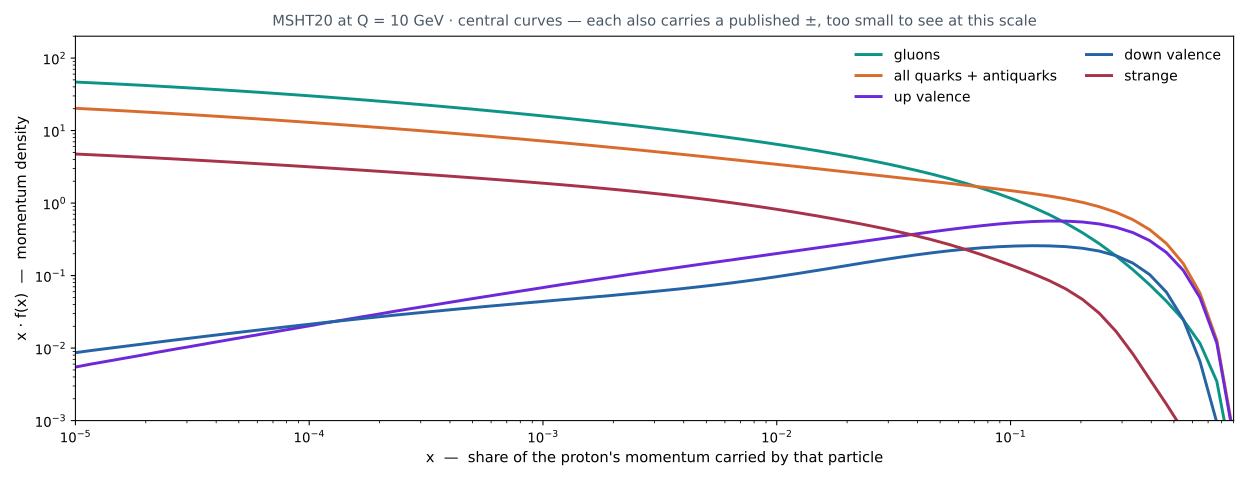
Each curve also carries a published ± of a few percent — 0.24% of the height of this plot, so it is not drawn. How that ± is arrived at, and how much the choice of method changes it, is the subject of this deck.

x2 · Q² is the probe, not the proton — it sets how finely you resolve; evolution redistributes momentum, never adds any

Speaker notes

Two confusions to head off. First: readers assume f(x) is bounded by 1 and are derailed when x·f reads 10 at x = 10⁻⁴ (f = 100,000 there). Second: on a log axis the small-x tail looks dominant but contributes little.

Bands are deliberately not drawn here — MSHT20's gluon ± is a median 1.4%, invisible on a 5.3-decade axis. Drawing it would suggest proton uncertainties are tiny and settled, which is the opposite of the setup. Uncertainty arrives on the next slide, where it is legible.

If asked about Q²: boosting the proton changes nothing — x is a ratio, so it is boost-invariant. The total momentum stays exactly 1 at every scale.

the problem — the ± is a choice

The groups agree on the proton. They do not agree on the error bar

three published sets: central values agree, band widths do not

PUBLISHED REFERENCEMSHT20 · CT18 · NNPDF4.0 released grids, all converted to a common 68% confidence level

left — the valueCentral curves lie on top of each other; the worst separation anywhere is about 3σ.

right — the ±The same groups' error bars differ by up to 3× on the gluon, from prescription alone.

what Colibri doesOne program, plug-in model, three prescriptions on one identical fit — a measuring instrument for methods, not a rival fitting group.

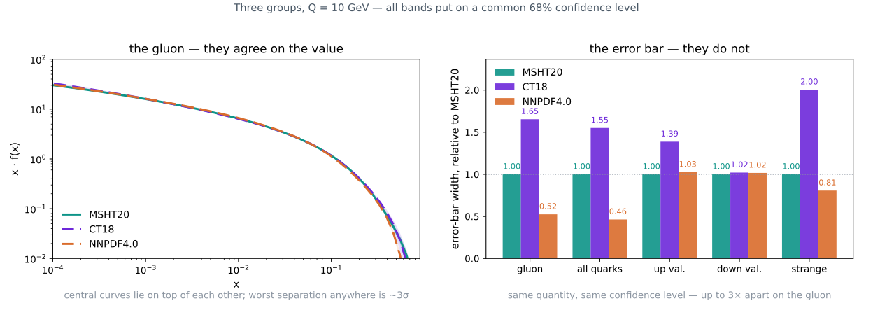
Comparing published sets can never isolate the recipe: the groups also differ in data, model and code.

x3 · Colibri — Costantini, Mantani, Moore, Schütze Sánchez, Ubiali · EPJC 86 (2026) 22

Speaker notes

This is the slide that motivates the whole project. The recipe's effect was structurally unmeasurable until one code could run all three on the same fit.

the problem — the three recipes

Three prescriptions, three distinct failure modes

Hessian

Does: measures the curvature of χ² at the minimum and inverts it.

Assumes: a positive-definite bowl.

Fails when: a flat direction gives zero or negative curvature — H⁻¹ is then meaningless. Not a wide band: no band at all.

Monte-Carlo replicas

Does: refits many noisy copies of the data; the spread is the uncertainty.

Assumes: frequentist scatter = uncertainty.

Fails when: refits roll to the prior bound — it then measures the box, not the data.

Bayesian

Does: maps the posterior by sampling; the spread is the uncertainty.

Assumes: a prior, and a converged sampler.

Fails when: sampling is under-converged — it reports a spuriously tight band.

in the well-constrained limitAll three provably agree. Confirmed twice here — the 13-parameter benchmark and the Phase-0 toy.

so agreement is a symptomNot a requirement. It tells you the problem is well-posed.

and disagreement is a signalIt means the question has gone ill-posed — not that the analysis is broken.

x4 · each failure mode is qualitatively different — that matters more than which band is widest

Speaker notes

Insist on the Hessian wording: it does not give a wide error bar, it gives none. The covariance is not positive-definite; there is nothing to quote.

the problem — scope

What I actually ran

the setup

parametrisation	MSHT20 — 52 free parameters, 4 analytic sum rules
framework	Colibri — JAX, auto-differentiable likelihood
data	full-DIS: 19 datasets, ≈3,092 points after cuts
which data	SLAC, BCDMS, NMC fixed-target F₂; HERA NC/CC; CHORUS, NuTeV ν-DIS
theory	FK tables, theoryid 40000000, t₀ covariance
starting scale	Q₀ = 1.65 GeV
runs	28 experiments, pre-registered criteria, one ledger

why nobody had seen this

Colibri's published demonstration used a 13-parameter benchmark with no flat directions. In that regime all three prescriptions agree — as they must.

My job was to take it to a realistic parametrisation, where the degeneracy is real. The problem only becomes visible at that data-to-parameter ratio.

The rigid 13-parameter form floors at χ²/N ≈ 5.6 on this data; MSHT20 reaches χ²/N ≈ 1.0, ΔlogZ ≈ +1450. The realistic model is not optional — it is the only one that fits.

Scope: this is a DIS-only study. Every statement here is about methods at this data-to-parameter ratio — not about MSHT20's published global fit.

x6 · 52 parameters · ≈3,092 measurements · 28 runs · the obstacle: 12 of 52 directions unconstrained

Speaker notes

The scope caveat matters. Do not let it be read as a criticism of MSHT20's released uncertainties.

the evidence — control

First: the machinery is correct. Without this, divergence is indistinguishable from a bug

closure test: three methods bracket the planted truth where data is strong

KNOWN-TRUTH TESTwe invent a proton, generate data from it, and fit that — so the right answer is known

where the data is strongAll three methods bracket the planted truth. Black dashed = the truth.

on an exactly solvable toyAgainst an answer computable in closed form: Hessian 0.99×, Monte-Carlo 1.00×, Bayesian 0.97×.

and the port itselfMSHT20-in-Colibri passed a 96-check parity gate to ≲10⁻⁹ — which caught a hidden ×A_g factor invisible at published parameter values.

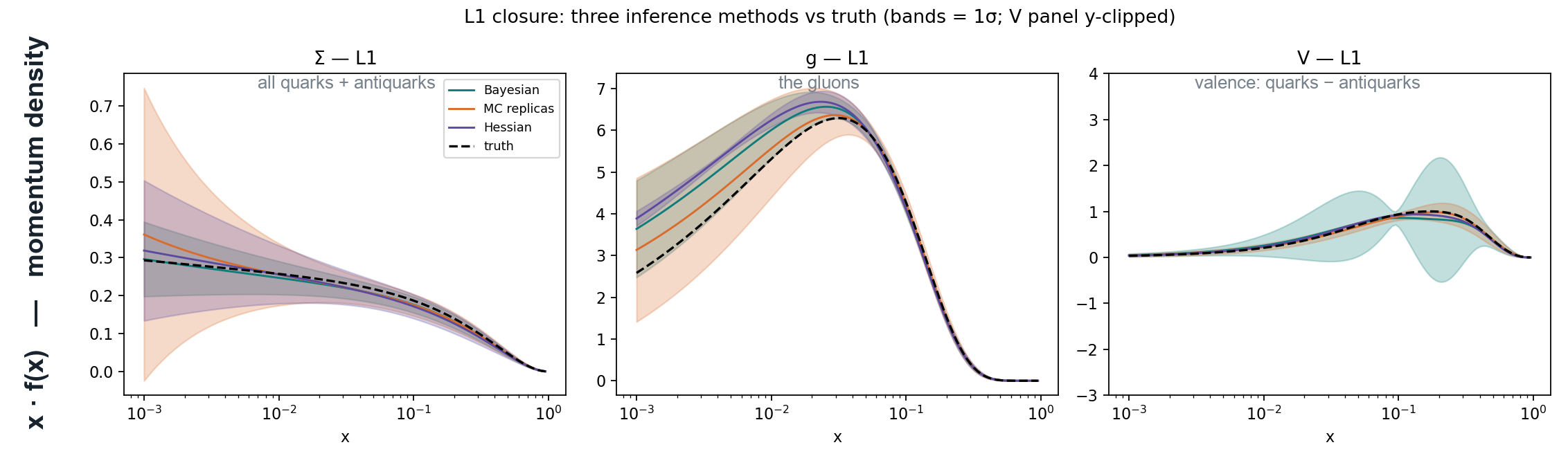
The implementations are right. Everything that follows is therefore physics, not a coding error.

x7 · closure = truth known · this slide licenses every later claim

Speaker notes

If she challenges the whole result, this is the slide to return to. The methods were validated where they should agree, before being trusted where they do not.

the evidence — the cause

The degeneracy is measured, not asserted

what a flat direction is — check it by hand

Two unknowns, one measurement that sees only their sum: total = 10.0 ± 0.5. (5,5), (2,8) and (8,2) all fit identically; (7,5) is off by four error bars. Moving along the sum is free; moving across it is not.

The data has no opinion about the split — so the prescription supplies one.

what this measures

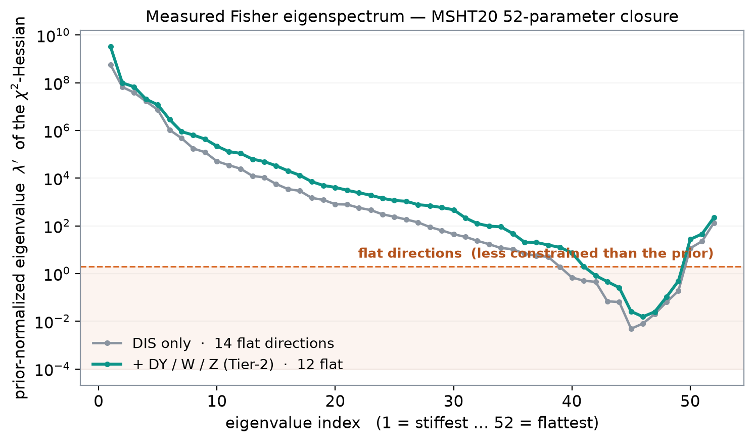
The Fisher information spectrum at the planted truth — how sharply the data pins down each independent direction. Noise-free, so this is geometry, not luck.

what it says

12 of 52 directions unconstrained on DIS. Spectrum spans ~11 orders of magnitude. Flattest: s−s̄, then strange sea, then high-x down-valence.

does more data fix it?

Adding Drell–Yan, W and Z moves it from 14 to 12. Two directions. An independent earlier analysis found 16→12 at condition ≈10¹³ — the same partial-cure conclusion.

x7 · control: pinning 15 high-order coefficients removes the worst flat directions · measured, not assumed

Speaker notes

Emphasise "measured". The strange sector was identified by the Fisher analysis independently of the coverage result on slide 11 — two routes to the same place.

the evidence — the main result

Same model, same data, only the recipe swapped: error bars 12–144× apart

what a ratio meansMeasure the width of the Monte-Carlo band, measure the width of the Bayesian band, divide. Same fit, same data — only the prescription changes.

the flavour combinationsΣ = all quarks + antiquarks · g = gluon · V = quarks − antiquarks · T8 = strangeness-sensitive. QCD evolution keeps these separate.

the numbersΣ 144× · g 80× · V 12× · T8 33× — Bayesian ±4% on the gluon where Monte-Carlo says ±300%.

REAL DATAfigure shows the SLAC+BCDMS subset, 648 points · the 12–144× ratios are the full-DIS fit

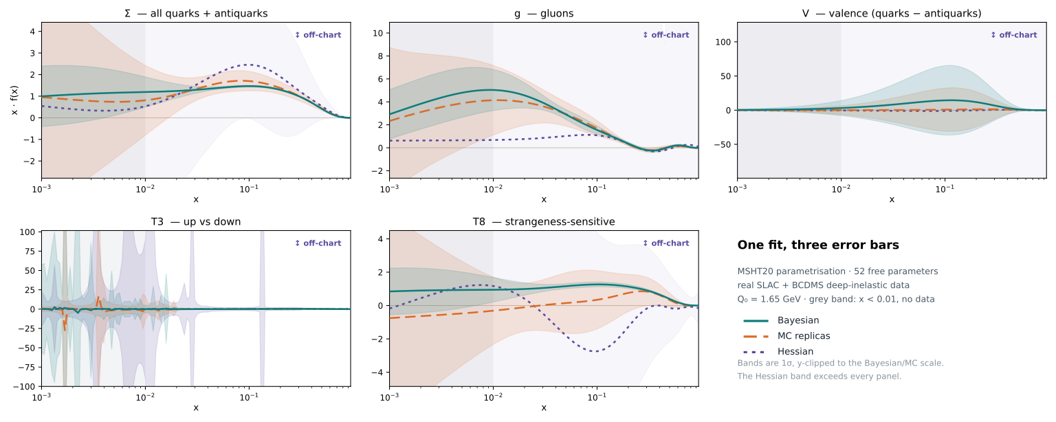
The Hessian does not give a wide band — it gives none. On real data its curvature matrix has condition ≈ 6×10¹¹: inverting it is numerically meaningless, so there is nothing to quote. (An earlier version also cited “10 of 52 negative eigenvalues”; that count sits at the finite-difference resolution limit. The condition number is the argument and is unaffected.)

x9 · PPDF-28, blind — the comparison metric was committed to version control before unsealing

Speaker notes

Be ready for "which dataset?" — the 12–144× is the full-DIS fit; the five panels are the 648-point subset, where the ratios are smaller. Both are in the ledger.

Note also 11/52 negative eigenvalues appears in an earlier run (PPDF-14). The 10/52 quoted here is the real-data blind result.

the evidence — the correction

I built the test that could have destroyed the headline, and ran it

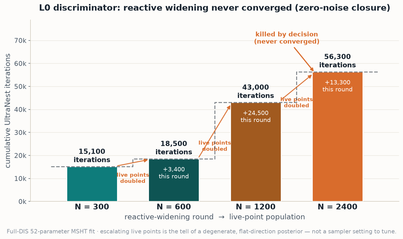
sampler effort doubled four times without settling

what I withdrew

My first result claimed Bayesian bands collapsing to ~2% of the PDF value. That was a sampling artefact at ESS ≈ 24.

how I know

Coverage climbed 6.5% → 49% → 51%, then went flat. Naive run: ESS ≈ 8, 262/400 divergences. Converged: ESS median 226, 41/3000 divergences, R̂ < 1.05.

Saturation is the proof: ESS 51 → 226 moved coverage by under 2 points.

and independently

A converged real-data run on a different machine with a different initialisation (ESS ≈ 181) reproduced the earlier band exactly.

The dramatic magnitude did not survive. The divergence did. Both are in the ledger, with dates.

x10 · left: nested sampling, effort doubled four times, never settling

Speaker notes

Do not soften this slide. It is the strongest evidence of good faith in the deck.

the verdict — which method to trust

Closure testing turns disagreement into a verdict

closure coverage by flavour against the 68% nominal

KNOWN-TRUTH TESTclosure only — coverage can only be measured where the truth is known

converged BayesianMean 57.9% against a nominal 68%, gate ≥55% — essentially calibrated. This is the recommended choice.

Monte-CarloOver-covers by 2–5×. Never wrong, because the band is too wide to be useful.

HessianUnusable in raw form — no positive-definite covariance exists to quote.

the one that still fails — and the honest caveat

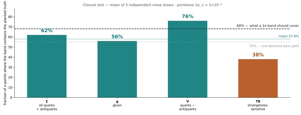
T8 covers 38%, failing 4 of 5 draws and reaching only 32% at the best convergence — the same sector the Fisher spectrum flagged independently. But the strange directions also carry the lowest per-direction sampling (ESS ≈ 10–58), so physical versus numerical is not yet fully separated.

x11 · 5-draw mean · single-draw coverage swings 47%↔76% and must never be quoted alone

Speaker notes

If asked whether 57.9% vs 68% is a failure: no — it is inside the pre-declared gate and within draw scatter. The robust signal is T8, which fails 4 of 5 draws.

the verdict — established, open, next

What stands, what does not, and what I need

established

in this deck

The three prescriptions genuinely diverge, 12–144× on real data.
The cause is a measured degeneracy — 12 of 52 directions, worst in strangeness.
Closure adjudicates: the converged Bayesian is the one to use.
An over-claim of mine was caught and withdrawn by my own test.

Two transferable results, easy to miss: nested sampling cannot converge on this posterior — 300→2400 live points, 15.1k→56.3k iterations, ESS = 1 after five days, while Fisher-preconditioned NUTS converges in an hour; and single-draw closure coverage cannot be trusted — 47%↔76% from noise alone.

open

not established

The Hessian was never given its production form — real fits regularise; mine did not.
The Tier-2 sweep came back under-converged (ESS ≈ 30), so "more data" is unresolved.
One functional form only; prior widths unscanned.
The real-data verdict is transferred from closure — there is no external anchor on real data.

2 · A fair Hessian rematch — score the regularised version production fits actually use.

3 · The ask: ν-DIS dimuon and W+charm FK tables, to constrain strangeness directly rather than inferring it.

What I would most value from you: whether the strange result is worth pursuing, and which of these to run first.

x12 · partonmap.com · full 27-slide read-out, results ledger and interactive explorer online

Speaker notes

End on the ask, not the result. She is the one who can judge whether the strange residual is physically interesting.