Research read-out · 20 July 2026 · internal · with M. Ubiali
Is the choice of uncertainty method a free choice?
Proton PDFs carry an error bar, and there are three standard ways to compute it —
Hessian, Monte-Carlo, Bayesian. In the well-behaved limit they agree. We stress-test them where the model is
more flexible than the data can constrain, and ask whether the answer now depends on which method you pick.
The claim we test
Under a parametrisation degeneracy the three methods diverge by orders of magnitude, each failing in a characteristic way — so the method is not a free choice.
How we test it
Closure tests with a planted, known truth (so error bars can be graded), a validated toy, then the real proton — all pre-registered, blind on real data.
Verdict so far
Largely confirmed — the divergence is real and mechanistic; a converged Bayesian is the reference. One earlier over-claim was corrected; the strange sector stays open.
52
free parameters (MSHT20 form, re-impl. in Colibri)
12–144×
inter-method spread on real DIS data
6
pre-registered phases · 3 complete, 1 partial
The head · what we're doing & why
PDFs are inferred, not measured — and their error bars flow into every LHC result
A proton parton distribution function (PDF) is the map of how the proton's momentum is shared among quarks
and gluons. It is never observed directly: it is fit to thousands of scattering measurements. The fit's error
bar is therefore a modelling choice — and it propagates into every cross-section prediction at the LHC.
The model. MSHT20 describes each flavour with a flexible functional form — 52 free parameters in total (Chebyshev polynomials × an xa(1−x)b shape), re-implemented in the JAX framework Colibri so the likelihood is auto-differentiable.
The data. Full-DIS: 19 datasets ≈ 3 092 points (SLAC, BCDMS, NMC, CHORUS, NuTeV, HERA), with the full experimental + theory (t₀) covariance.
The tension. 52 parameters is more freedom than DIS data can pin down. Some parameter combinations are barely constrained — and there the error bar stops being a fact about the data and starts being a fact about the method.
Why it matters. If two accepted methods disagree by 100× on the same data, then quoted PDF uncertainties — and everything downstream — depend on an arbitrary choice.
The inference chain. Data constrain the 52 parameters; the parameters' remaining freedom becomes the PDF error bar. Our question is entirely about that last step.
All three methods start from the same χ² fit to the same data. They differ entirely in
how they summarise the uncertainty around that fit — and in the well-behaved limit they agree. Everything
in this deck is about what happens to each when that limit breaks.
1 · Hessian
Laplace / linear error propagation
cheapest · one fit
Idea
Approximate the posterior as a Gaussian centred at the best fit.
Construction
Minimise χ²; take the curvature H = ½ ∂²χ²/∂θ∂θ; parameter covariance = H⁻¹; band σ_f = √(Jᵀ H⁻¹ J). Production inflates by a tolerance T².
Assumes
A single, well-defined, positive-definite minimum (a locally quadratic χ²).
Fails when: a direction is flat or curved → H has zero / negative eigenvalues → H⁻¹ blows up or is imaginary. No valid band.
2 · Monte-Carlo
replica ensemble
N full fits · expensive
Idea
The uncertainty is the spread of fits to many noisy copies of the data.
Construction
Make ~100 pseudo-datasets D_k = D + η_k, η_k∼N(0,C); refit each → band = std of f(x) across replicas.
Assumes
The estimator's frequentist scatter equals the uncertainty (exact only in the linear-Gaussian limit).
Fails when: along a flat direction the replicas scatter to the parameter bounds → bands far too wide (over-covers).
3 · Bayesian
full posterior
most expensive · exact
Idea
Keep the whole posteriorP(θ|D) ∝ L(D|θ)·π(θ); the band is its spread.
Construction
Sample the posterior (nested sampling, or gradient NUTS); band = std of f(x) over the samples.
Assumes
A prior π(θ) (here bounded-uniform) — and that the sampler actually converges.
Fails when: where the data is silent the band is prior-limited; a non-converged sampler under-explores → collapses (over-confident).
The point of the whole study: in the well-constrained Gaussian limit these three coincide, and their differences are ignored in practice. We ask whether that assumption survives a degenerate parametrisation — because if it doesn't, the quoted PDF uncertainty depends on a choice, not the data.
The head · the exact statement
The falsifiable statement — and the closure test that lets us grade it
We turn a vague worry (“methods might differ”) into something we can prove or disprove: a
pre-registered, falsifiable hypothesis, tested where the true answer is known by construction.
Hypothesis (pre-registered)
Under a degeneracy, the three error bars satisfy
σ_Hessian — undefined (curvature indefinite)
σ_Bayes ≪ σ_MC (diverge by ≫ 2×)
and closure coverage grades Bayes as the reliable one.
Falsifiable: if all three agree within ~2× and cover truth equally, the hypothesis is wrong.
The grading metric — coverage
coverage(f) = fraction of x where
| f_fit(x) − f_true(x) | ≤ σ_f(x)
Per flavour f ∈ {Σ, g, V, T8}, for x > 5×10⁻⁴. Nominal for a 1σ band ≈ 68%; pre-declared pass gate ≥ 55%. Only possible because closure gives us f_true.
Real data has no known answer, so methods can't be graded on it directly. A closure test manufactures one:
1
Plant a known truth
Fix the 52 parameters to the published MSHT20 values — now f_true(x) is known exactly.
2
Generate pseudo-data (level-1)
Take the theory prediction at truth and add one draw of realistic experimental noise: D = T(θ_true) + η, η∼N(0,C).
3
Fit it three ways
Run Hessian, Monte-Carlo, and Bayesian on the same pseudo-data → three error bands for each flavour.
4
Grade against the planted truth
Measure coverage; repeat over independent noise draws so the score isn't a fluke of one dataset.
The problem · root cause
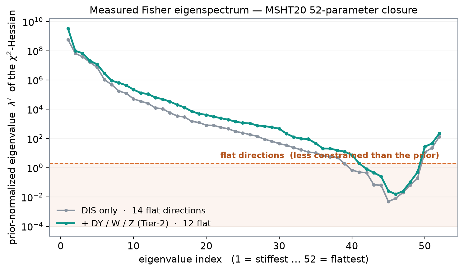
The Fisher eigenspectrum: a tail of near-zero eigenvalues, dominated by the strange quarks
Why would well-established methods disagree at all? Because the information matrix has directions the data
barely sees. Diagonalise the curvature of χ² at the truth and the smallest eigenvalues are the degeneracy —
and they point at the strange sector.
The measured spectrum — prior-normalized χ²-Hessian eigenvalues at truth, computed fresh for this deck. An ~11-order-of-magnitude range and a tail of 12 flat directions (DIS only), only partly lifted to 9 by DY/W/Z. (Counts corrected 6 Aug 2026 by exact re-measurement; the plot above is the original forward-difference spectrum, kept as the record of what this deck computed at the time.) Condition number ≈ 10¹¹ — a severely degenerate fit.
What a flat direction is
H_ij = ∂²χ² / ∂θ_i ∂θ_j |_truth (Fisher info)
eigenvalue λ_k → 0 ⇔ a parameter
combination the data can't constrainAlong such a direction the fit can move far at almost no χ² cost. The Hessian band σ = √(Jᵀ H⁻¹ J) then blows up or — off the exact minimum — goes imaginary.
The flattest directions are strange. #1 rho_* (the s−s̄ asymmetry, σ 125→51), #2 sp_* (the strange sea, 56→28), then high-x d-valence.
More data helps but doesn't cure it. Adding Drell-Yan / W / Z stiffens the fit, yet 12 of the 14 flat directions remain and the condition number is unchanged (~10¹¹) — a real but modest, partial cure.
It's the model, not the data. Pinning 15 high-order Chebyshev coefficients removes the 5 worst flat directions → the degeneracy is genuine excess flexibility.
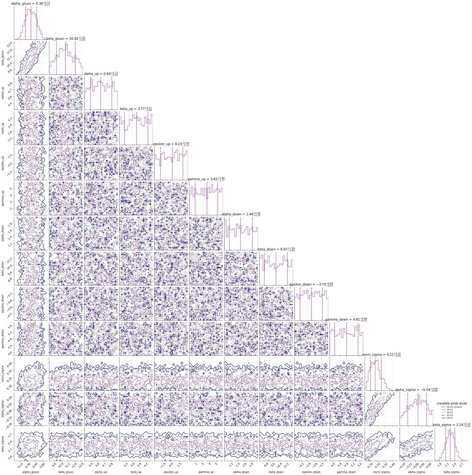
The degeneracy in parameter space — posterior corner plot (reduced-model closure). Many marginals are flat (the data doesn't move them) and most 2-D panels show no correlation; only αgluon, βgluon and the σ-shape are pinned. Flat marginals = flat directions.
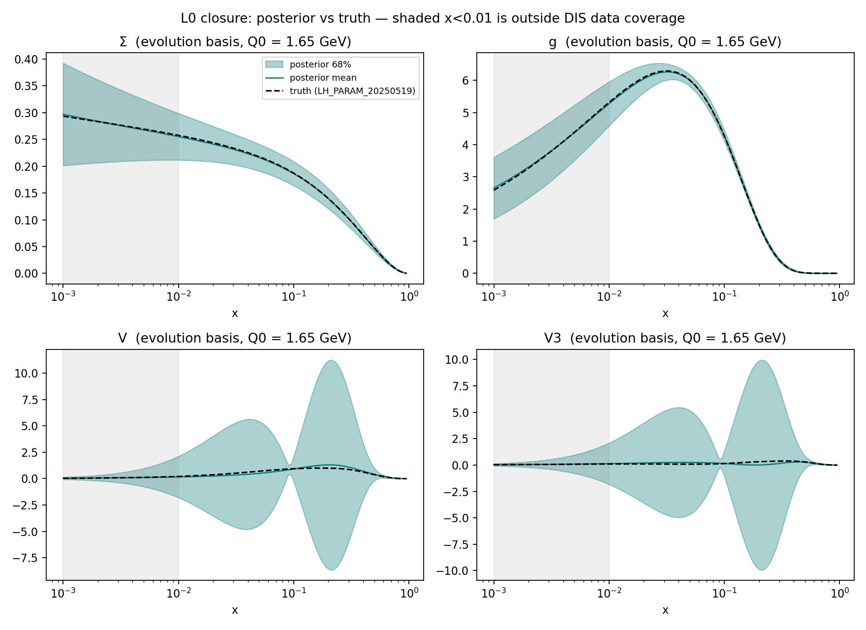
…and the same degeneracy in the PDF (PPDF-2). The posterior recovers truth (dashed) for Σ and g — but the valence V, V3 bands balloon to ±10× the PDF: the flat directions drawn out in the fit itself.
Where we are
A six-phase, pre-registered program — 3 complete, 1 partial, 2 open
Ordered falsification-first: the cheap steps that could kill the conclusion run before the expensive
confirmations. Every phase has a written goal, gate, and falsification criterion fixed before the numbers.
Phase 0
Validate the instrument
✓ PASS
PPDF-24
decisive
Phase 1
Convergence: real or artifact?
✓ DONE
PPDF-25
Phase 2
Degeneracy sweep
◑ PARTIAL
PPDF-26
Phase 3
Fair Hessian rematch
○ PENDING
PPDF-27
Phase 4
Real proton (blind)
✓ DONE
PPDF-28
Phase 5·6
Physical cure · paper
○ DEFERRED
PPDF-29
0 → validate. Prove the three method implementations are correct against a known answer, so later disagreements are physics.
1 → the decisive fork. Separate a sampling artifact from a real posterior property — this reshapes everything after it.
4 → real data, under a blind, pre-declared metric. The physics deliverable.
2 partial (Tier-2 fit under-converged); 3 & 5 open — the fair-Hessian rematch and the physical strange cure.
Foundation · PPDF-1…6
Before the stress-test: the tools are validated, and in a benign closure all three methods track the truth
Two things had to hold before any disagreement could mean something. First, our Colibri
re-implementation must reproduce the published MSHT20 fit. Second, in a well-constrained closure the three
methods must agree — with each other and with the planted truth. Both hold — and the very first cracks already
show where the data thins.
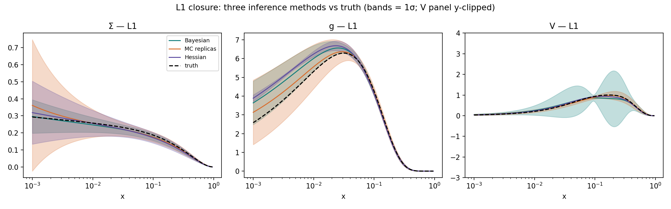
L1 closure — the three methods (Bayesian teal, MC orange, Hessian purple) vs the planted truth (black dashed), for Σ, g, V. All three bracket the truth in the data-rich region; the bands differ in width, and in V the Bayesian already balloons where the valence data thins.
Replication (PPDF-1…5). Colibri reproduces MSHT20 predictions and the published closure-test table — parity gates passed to the reference implementation (a hidden ×Ag factor was caught and fixed along the way).
Posterior recovers truth (PPDF-2). The Bayesian posterior mean sits on the planted truth for Σ and g to sub-percent; the fit machinery is sound.
Methods agree — when constrained (PPDF-6). For Σ and g the three bands overlap and contain the truth. This is the “everyone agrees” baseline the rest of the deck departs from.
The first crack. In V, where DIS data is thin, the bands already start to diverge — a preview of the degeneracy we dissect next.
Why this matters: it rules out the boring explanation. When the methods diverge later, it is not because our code is wrong or the fit is broken — the same code agrees with truth here.
The evidence · Phase 0
Before claiming the methods disagree, we prove the tools are correct
The headline is that three methods diverge. Before that means anything we must exclude the boring
explanation — a bug in our Colibri re-implementation. So we run all three on problems whose true error bar is
known exactly, and watch them pass when it's easy and fail mechanistically when it's degenerate.
The analytic toy (exact truth)
−2 log L(a,b) = (a−â)²/s_a²
+ ( b − b̂ − κ(a−â)² )² / s_b²
A curved “banana” valley in (a,b) inside a bounded prior; the exact posterior is computed by grid. One knob — the constraint s_a on a — dials the degeneracy from mild to extreme. Then repeated on the full 52-param MSHT20 closure.
Left: the validation gate — all three recover the exact band to ≤3%. Right: cranked to an extreme flat valley, each fails in its own way.
Three failure modes — and, crucially, why each happens:
Hessian → indefinite (2 negative eigenvalues). At a fit sitting off the exact minimum in a curved valley, the χ² acquires wrong-sign curvature; H⁻¹ is not positive-definite, so no band exists — a breakdown, not imprecision.
Monte-Carlo → 1.32× truth, with 81% of replicas pinned at the prior bound. Along the flat direction the noisy re-fits wander until the prior stops them, so the spread measures the prior width, not the data.
Bayesian → 0.19× (5× too narrow) at ESS 22 when rushed — but 0.93× at ESS 221 when converged. A short sampler can't traverse the curved geometry, under-explores, and reports a spuriously tight band. This failure is fixable by convergence.
The structural insight: two failures are geometry (Hessian, MC) and are irreducible; one is sampling (Bayesian) and is curable. “Is a given divergence geometry or sampling?” is exactly the question the rest of the analysis answers.
The evidence · Phase 1 (decisive)
Is the Bayesian “collapse” a real posterior property, or just a sampler that hasn't converged?
This is the fork the whole result turns on. If the collapse is a sampling artifact, our earlier scary
headline was wrong; if it survives genuine convergence, it's physics. To decide it we first had to make the
sampler actually converge on a cond ≈ 10¹³, 52-D posterior — which standard nested sampling cannot.
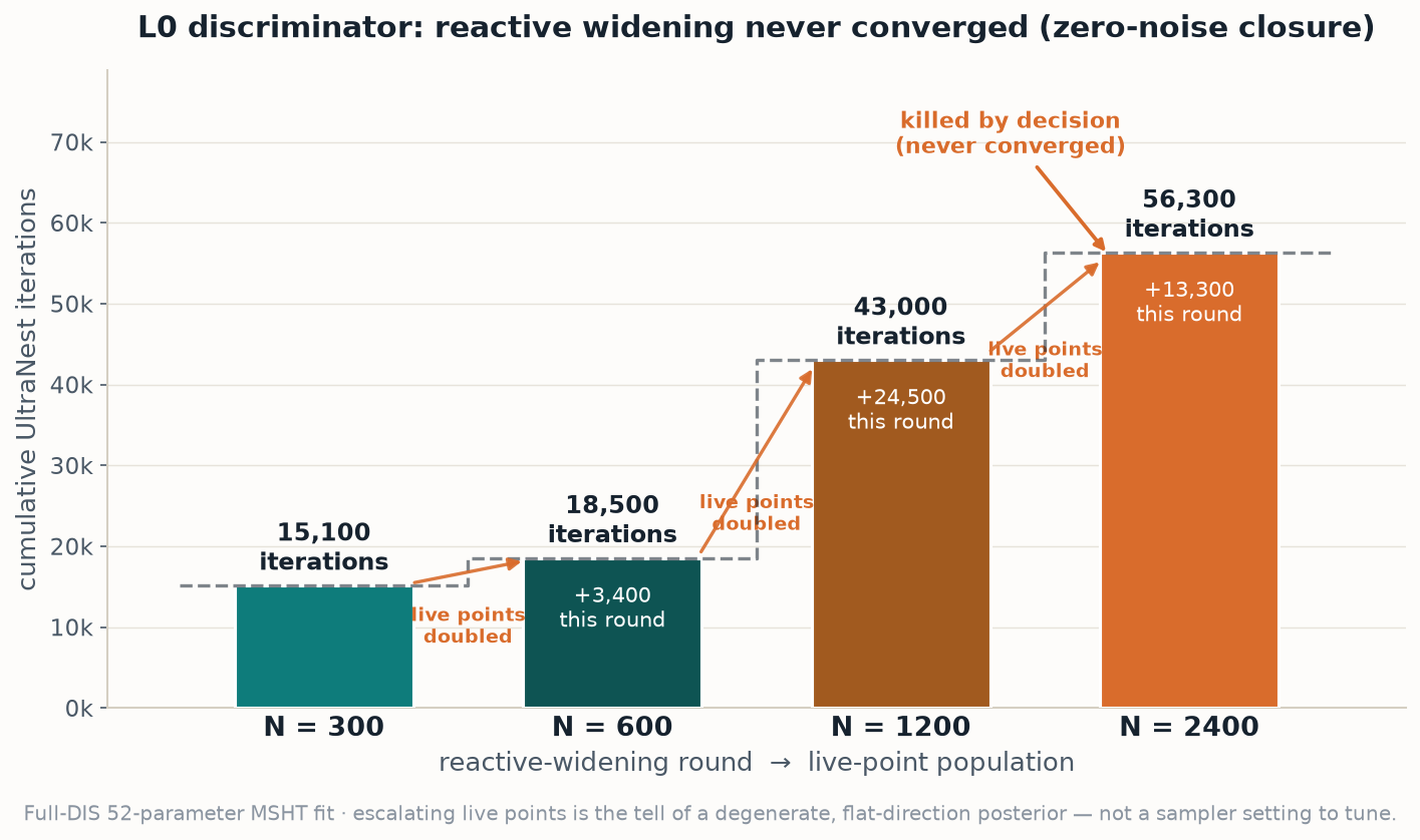
Nested sampling never converges (PPDF-16). Doubling the live points just escalates the iteration count (15k → 56k) and never settles — the signature of a flat, degenerate posterior, not a knob to tune. This is why we switched samplers.
Coverage climbs, then flattens. From ESS 51→226 (4× the sampling) coverage moves <2 points — the band has converged, so the residual shortfall below 68% is not fixed by more computing.
The sampler fix. Nested sampling stalls (ESS=1). Gradient-based NUTS with a Fisher-preconditioned dense mass matrix — i.e. we hand the sampler the degeneracy's geometry — converges in ~an hour.
Rushed vs converged. A naive short run gives ESS 8 with 262/400 divergences and 6.5% coverage — pathological. A proper run reaches ESS median 226 (min 58), 41/3000 divergences, R̂ < 1.05, and coverage ~51%.
The verdict on the fork. The gross collapse (2%-of-truth bands) was a sampling artifact — convergence cures it. But coverage saturates ~51%, below the 68% ideal, so a genuine, modest shortfall remains.
Reading the diagnostics
ESS — independent-sample equivalent (mixing)
div — NUTS trajectory failures (bad geometry)
R̂ — between/within-chain variance; ≈1 = converged
All three must be healthy at once before a coverage number is trustworthy.
The evidence · Phase 1
One dataset isn't enough: coverage is noise-dominated — but the strange sector really does under-cover
A single pseudo-dataset is one roll of the dice. To separate a real shortfall from bad luck we fit
five independent noise draws to convergence and average. The spread is large — and, tellingly, it does not
track how hard we computed, which proves the runs are converged and the scatter is the data.
Coverage swings 47→76% from the noise alone. Draw 3 (ESS 34) beats draw with ESS 89 — coverage is uncorrelated with ESS, so these are converged; the scatter is the pseudo-data.
Σ, g, V are ~calibrated (56–76%). T8 (strange) = 38% — fails 4 of 5 draws and stays at 32% even at the highest ESS. This is the one place the converged Bayesian is genuinely over-confident.
What this pins down: the average converged coverage is ~58% — just under nominal, not the catastrophic collapse we first reported. The only robust deficit is localised to the strange sector — exactly the flattest direction from slide 4.
The evidence · Phase 4 (blind)
On the real proton, the three methods diverge 12–144× — and it is not a convergence artifact
The metric was written down and committed before the real data was unsealed. The decisive control:
the fully-converged real-data Bayesian band equals the earlier ESS≈24 band — so the narrowness is the true
posterior width, not under-sampling. The divergence is therefore real.
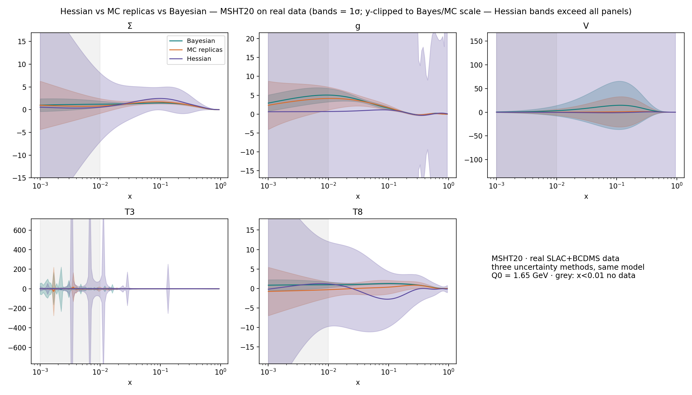
The real result — the three methods as 1σ PDF bands, real MSHT20 data, five flavours. Bayesian (teal) is tight; Monte-Carlo (orange) is wide; the Hessian (purple) bands blow past every panel and go wild in T3 / T8 — the strange sector. Same model, same data: the error bar is set by the method.
Bayesian (converged) 2–17% vs Monte-Carlo 200–550%, per flavour, on the same data. The Hessian gives no bar at all: 10 of 52 eigenvalues negative, cond ≈ 6×10¹¹.
The cross-check that settles it. The converged run (ESS 181, 80/3000 div) reproduces the sealed ESS≈24 band on a different machine to within its width → the narrowness is the genuine posterior, not under-sampling.
Monte-Carlo over-covers (200–550%) — replicas fill the flat valley to the prior bounds, exactly as the toy predicted.
Hessian breaks — an indefinite curvature matrix has no positive-definite inverse, so there is no valid Gaussian error at all.
Where they diverge most tracks the physics: largest in T8 / Σ (strange-adjacent), smallest in valence — the same ranking as the Fisher spectrum.
Have we proven it? Largely yes — with one claim we corrected ourselves
Reconciling closure (known truth) with real data gives a sharper, more defensible statement than the one
we started with. The core thesis holds; the most extreme version of it did not.
✓ Proven
✓ The three methods genuinely diverge (12–144×) — on closure and real data; not numerical noise.
✓ Each failure is mechanistic and reproduces against a known answer (Hessian indefinite, MC to the prior bound, Bayesian sampling-collapse).
✓ Graded by closure coverage, the converged Bayesian is the reference (~58%); MC over-covers; Hessian breaks.
⚠ Corrected · ○ not yet proven
⚠Corrected: the earlier headline (PPDF-23) of a 2%-of-truth Bayesian collapse and “12–144×” was convergence-confounded (ESS≈24). The divergence is real, but that extreme magnitude was inflated — retracted.
○ Is the strange-sector under-coverage physical, or residual under-exploration of the flattest direction? Not yet closed.
○Generality beyond the MSHT parametrisation — untested.
○ A fair, regularised Hessian (the production trick) may partly rescue that leg — not yet run.
Intellectual-honesty note. Phase 1 (closure) briefly tempted us to conclude “the whole divergence is an artifact.” Phase 4 (real data) showed that was too strong — only the catastrophic collapse is an artifact — and we revised the claim in writing rather than let it stand.
The tail · what's missing
What's missing — and the four calls to make with Maria before this is a result
The gaps are specific and mostly decision-shaped, not open-ended. Each has a concrete next experiment
and a lean; none of them overturns the core finding, but they are what turn “strong internal result” into “paper.”
1 · Is the strange residual physical?
T8 under-coverage (38%) could be a genuine prior-limited posterior in the flattest direction — or residual under-mixing (strange parameters still have the lowest per-direction ESS, ~10–58).
Lean: physical — but confirm with per-direction mixing diagnostics + a strange-targeted long run.
2 · How do we adjudicate real data (no truth)?
We currently transfer the closure verdict. Should we add an external anchor — consistency of central values and bands with published MSHT20 & NNPDF4.0 in the well-constrained regions?
Lean: yes — anchor to published PDFs as a calibration check.
3 · How much is prior-driven?
Where the data is silent, the Bayesian band is set by the (bounded, uniform) prior, and MC by the same bounds. Part of the divergence is a prior statement, not a data statement.
Lean: add a prior-width sensitivity scan; report flat-direction bands as prior-conditional.
4 · Does it generalise?
Is “converged Bayesian as reference, Hessian & MC as cross-checks” defensible guidance — and does the pattern hold beyond the MSHT functional form?
Lean: yes for MSHT-in-Colibri; test on a neural-net (NNPDF-style) parametrisation before claiming it broadly.
Where we go next
Next analyses — from finishing the sweep to the physical cure
Two are compute we can finish now; the decisive physics step needs new data — the one place the program
depends on the collaboration, not the cluster.
Phase 2 (finish)
Whitened, fully-converged Tier-2 closure at 2–3 degeneracy levels → the coverage-vs-degeneracy law and the onset of divergence (the current run under-converged at ESS 30).
~3 h compute
Phase 3
Give the Hessian a fair rematch — regularised / dynamic-tolerance covariance (the production trick), plus profile-likelihood as an independent fourth method.
compute-light
Phase 5 · physics
Integrate ν-DIS dimuon (NuTeV/CHORUS) and W+charm FK tables → does pinning strange shrink the degeneracy and the divergence? A standalone result on the strange PDF.
needs data integ.
Generality
Prior-sensitivity scan; repeat on a neural-net parametrisation to test model-independence of the pattern.
scoping
Publication
Toy validation + convergence + fair method set + blind real-data → a methodology paper (hep-ph), with Maria.
on track
The tail · bottom line
Bottom line
The choice of PDF uncertainty method is not a free choice under a
parametrisation degeneracy. On the real proton the three standard prescriptions disagree by up to two orders of
magnitude — and closure tests with a known answer tell us which to believe.
Use a properly converged Bayesian as the reference. It is the only one that is calibrated (~58% coverage) where the data is degenerate.
Treat Monte-Carlo as conservative and the Hessian as invalid in the degenerate regime — MC over-covers, the Hessian has no positive-definite error at all.
Watch the strange sector — even the reference method is over-confident there, and that is the honest caveat on the whole result.
What changed our own mind. We began ready to report a dramatic Bayesian collapse. Convergence testing showed the extreme version was a sampling artifact; real data showed the divergence itself is real. The result is milder and sharper than we started with — and we can defend every number in it.
3 / 6
phases complete, 1 partial
1
headline corrected by us
Backup · methods & reproducibility
Methods & diagnostics
Quantity
Value
Parametrisation
MSHT20, 52 free params (Colibri re-impl., JAX)
Data
full-DIS, 19 sets ≈ 3092 pts; theory 40000000; t₀ covmat
Closure
level-1, planted truth = MSHT20 central values
Coverage
pointwise 1σ; Σ / g / V / T8; x > 5×10⁻⁴; gate ≥ 55%