Research read-out for Maria Ubiali · 1 August 2026
How well do we really know what is inside the proton?
A proton is not a single solid object — it is made of smaller particles, and the way they share the proton's
momentum has to be measured from experiments, not calculated from theory. The result is a set of curves
called parton distribution functions. Every prediction made at the Large Hadron Collider depends on
them, and on the error bars attached to them.
the question
Those error bars are not measured — they are computed, and there are three standard ways
to compute them. The field assumes the three broadly agree. Maria asked me to check.
They do not.
the answer, up front
On real data the three disagree by up to 144× on the same quantity — a real effect, not a
numerical artifact. Against a known truth the converged Bayesian is the trustworthy one;
Monte-Carlo is over-conservative; the Hessian gives no valid band at all. One problem survives
even the best method: the strange quark.
1 · the context
Who produces these proton maps, why Maria's group built a new tool, and what she asked me to do.
2 · the physics
What is actually being measured, and where the error bar comes from.
3 · what I ran
Four weeks, 28 experiments — validating the tools and measuring the underlying problem.
4 · what I found
The three methods disagree sharply. One of them is right — and I can show which.
1 / 24partonmap.com · proton structure & uncertainty · with M. Ubiali, Cambridge
Speaker notes
Orientation first, no numbers yet. "This is the read-out on the project you set me in July. I'll do it in four
parts: the context, the physics, what I ran, and what I found."
If she wants the punchline immediately: the three uncertainty prescriptions differ by up to a factor of 144 on
real data, closure testing says the converged Bayesian is the trustworthy one, and the residual problem is the
strange sector.
1 · the context — my understanding of the programme
What I understand this programme to be
Proton structure, and how honestly we can state its uncertainty. Six points, in order:
1
What we are mapping
A proton is not one solid particle. It is a swarm of quarks and gluons sharing its momentum.
A parton distribution function is simply the curve saying how likely each one is to carry a given
share.
one curve per particle type · slide 7
2
Why anyone needs them
These curves cannot be calculated — the maths is intractable. They must be fitted to thousands
of experiments. Every prediction at the Large Hadron Collider then uses them as an input.
PDF × collision = prediction · slide 8
3
Who actually makes them
Four collaborations worldwide. NNPDF (“Neural Network PDF”, Europe), MSHT
(Martin–Stirling–Thorne–Watt, UK), CT (CTEQ–TEA, US), JAM (Jefferson Lab, US). Everyone else
downloads their results.
I use the MSHT proton model · slide 4
4
The problem: the ± is a choice
Each fit must also state how uncertain the curve is. That number is not measured — it is computed,
and there are three accepted recipes. Each group builds one recipe into its own software.
Hessian · Monte-Carlo · Bayesian · slide 10
5
What Maria's group built
Her Cambridge programme asks whether apparent “new physics” is really a mis-modelled proton. Her
group released Colibri — the first program that can run all three recipes on one identical
fit.
Colibri, 2025 · slide 5
6
What I am doing, and why it is hard
I put the real MSHT proton model into Colibri and ran all three recipes on the same fit. It is hard
because the model has more freedom than the data can pin down — so the recipes are free to
disagree.
we measure them differing by up to 144× · slide 16
2 / 241 · the context · the rest of this deck expands each of these six points in turn
Speaker notes
This is the "do I understand what I've been asked to do" slide. Walk the six in order; each one is expanded
later in the deck, and the card footers say where.
Expansions if she probes: NNPDF = Neural Network PDF collaboration (Italy/UK/Netherlands/Spain);
MSHT = Martin, Stirling, Thorne, Watt — the UK group whose 2020 set (MSHT20) I re-implemented;
CT = CTEQ–TEA (US); JAM = Jefferson Lab Angular Momentum (US).
The honest framing of point 6: the difficulty is not computational, it is that the question is genuinely
ill-posed along the directions the data cannot constrain — 14 of the 52 parameter-combinations.
1 · the context — how these curves are made, and by whom
The curves are fitted to data, not calculated — by four groups worldwide
There is no equation that gives these curves from first principles: the
maths of the strong force cannot be solved that way. So each curve is fitted — adjusted until it matches
thousands of past collision measurements. Only a handful of groups do this. Everyone else uses their results.
Group
What the letters stand for
Where
How they describe the proton
What they publish
NNPDF
Neural Network PDF
Europe
A neural network — a flexible computer model with no fixed shape
NNPDF4.0 — a central curve + ~100–1000 replicas
MSHT
Martin, Stirling, Thorne, Watt — four physicists' surnames
United Kingdom
A fixed algebraic formulathe model I use
MSHT20 — a central curve + ~60 error members
CT
CTEQ–TEA — a US theory-and-experiment project
United States
A fixed algebraic formula
CT18 — a central curve + ~60 error members
JAM
Jefferson Lab Angular Momentum
United States
A fixed algebraic formula
JAM sets — a central curve + replicas
so what is the actual deliverable?
Not a program — a data product. Each group publishes a
“PDF set”: numerical tables of the fitted curves, distributed through LHAPDF, the shared
library every collider analysis reads. Notice the pattern in the last column — the uncertainty recipe
decides the form of what they ship. Hessian groups ship a fixed set of error members; Monte-Carlo
groups ship an ensemble of replicas.
3 / 251 · the context · LHAPDF = the standard distribution format · the 2020 set “MSHT20” is the one I re-implemented
Speaker notes
The point to land: fitting is a modelling exercise, not a measurement, so reasonable people using the same
data get slightly different curves. That is normal and expected.
Deliberately left off this table: how each group computes the uncertainty. That is the next slide, and
it is where the real problem lives.
1 · the context — the three recipes, explained
What “the uncertainty band” is, and the three ways to compute it
SCHEMATICthe band is the honest statement of doubt — and it is computed, not measured
recipe 1
one fit · cheapest
Hessian
Measure how sharply the fit worsens as you step away from the best point. Steep walls mean a small
uncertainty; shallow walls mean a large one.
–Assumes one clean, well-defined best fit.
–Breaks if a direction is flat — the maths cannot be inverted.
recipe 2
~100 fits
Monte-Carlo replicas
Make about a hundred noisy copies of the data, re-fit every one, and take how much the answers
scatter as the uncertainty.
–Assumes the scatter of re-fits equals the uncertainty.
–Breaks if re-fits wander to the edge of the allowed range.
recipe 3
slowest · most complete
Bayesian posterior
Map out the whole range of settings the data permits, and read the spread of the resulting curves
straight off.
–Assumes a stated prior, and a sampler that finishes.
–Breaks if the sampler stops before exploring properly.
All three answer the same question by different logic — so when the data is decisive they agree, and when it is not, they need not.
4 / 271 · the context · each group historically built one recipe into its own code — see the previous slide
Speaker notes
Define the band first: it is not measured, it is computed from the fit, and it is the honest statement of how
much the curve could still move.
Technical detail if she asks: Hessian = second derivative of χ² at the minimum, band = √(JᵀH⁻¹J), inflated by
a tolerance in production fits. Monte-Carlo = resample the data within its covariance and refit; exact only in
the linear-Gaussian limit. Bayesian = sample the posterior P(θ|D) ∝ L·π; the only one that is exact for a
non-linear model, but it needs a prior and a converged sampler.
1 · the context — what Maria's group built, and why
One program that can run all three methods on the very same fit
Maria Ubiali leads a programme at Cambridge called Physics Beyond the
Standard Proton, funded by the European Research Council. Its worry: a hint of new physics at the collider
might really be the proton being mis-modelled. So the size of that band has to be trustworthy.
SCHEMATICwhat changed · Colibri released 2025 by the Cambridge group (Ubiali et al.)
Now you can hold the model and the data completely fixed and change only the method — so any difference you see is caused by the method alone.
5 / 251 · the context · Colibri arXiv:2510.03391 · the “programme” is Maria's ERC-funded project at Cambridge
Speaker notes
The scientific stake is why the plumbing matters: if the programme is going to say an LHC anomaly is or is not
new physics, the proton's uncertainty band has to be trustworthy rather than an artefact of which recipe was used.
Colibri is built on the existing shared data and theory infrastructure, so it is not a rival fitting group —
it is a measuring instrument for comparing methods. Its published demonstration used a simplified 13-setting toy
proton, where all three methods agreed.
1 · the context — what Maria asked me to do
What Maria asked me to do
Her brief, from our meeting and follow-up email (7–8 July 2026). The last line is what this deck answers.
1
Move from a toy model to a real one
Colibri had only been demonstrated on the 13-parameter Les Houches toy. Implement MSHT20 — “one of the most broadly used PDF sets in LHC phenomenology” — as a new Colibri model.
done
2
Start with data we already understand
Use the same DIS data as the earlier toy fits so the comparison is clean — then scale up.
done
3
Compare Hessian vs Monte-Carlo vs Bayesian uncertainties
Her stated final goal — the head-to-head that Colibri makes possible for the first time.
this deck
A real, widely-used parametrisation · real data · all three uncertainty methods under one roof.
4 / 241 · brief per M. Ubiali 7–8 Jul 2026 · MSHT20 parametrisation Eqs (2)–(8) of arXiv:2012.04684
Speaker notes
Say plainly that this is her question and I am reporting back on it. The novelty is not a new method —
it is the first like-for-like test: same parametrisation, same data, same code, three uncertainty prescriptions.
FPPDF (arXiv:2602.07118) released the MSHT20 parametrisation publicly; I used it as the reference to validate
my port against — that is where the 96-check parity gate comes from.
1 · the context — the whole project on one slide
What I did, and what came out
The published demonstration of Colibri used a simplified 13-setting toy
proton, and there all three methods agreed. I swapped in the real 52-setting proton form and compared
the methods on real data. Everything after this slide is the detail behind these numbers.
the model
52 settings
the real MSHT proton form, re-implemented — not the 13-setting toy
the data
3 092
real measurements of electrons and neutrinos scattering off protons
the work
28 runs
over four weeks — validating the tools, then the comparison itself
the obstacle
12 of 52
settings the data cannot pin down at all — mostly the strange quarks
SCHEMATIC + OUR RESULTleft: why the question is ill-posed · right: the spread we measure on real data
Where the data is silent, the method — not the measurement — decides how big the uncertainty looks.
6 / 261 · the context · closure tests then tell us which of the two survivors is right — part 4
Speaker notes
This is the "everything at a glance" slide — scope, obstacle, outcome — before the detail starts. If she only
remembers one slide, this is it.
The toy model in Colibri's paper had no flat directions, so all three methods agreed and the problem stayed
hidden. The real 52-setting form exposes it. That the worst directions are the strange quarks is a concrete,
checkable claim — it comes out of the information analysis in part 3, not from assumption.
Careful wording: 12–144× is our measurement, not a textbook number. The Hessian does not merely give a
wide band — its maths breaks down and returns no valid band at all.
2 · the physics — what we are talking about
A proton is not one particle — it is a swarm of quarks and gluons
3 valence quarks (u u d) — these give the proton its identity
gluons — they bind it together, and carry about half its momentum
the sea — short-lived quark–antiquark pairs, including strange
collectively these are called partons
SCHEMATICa picture of the constituents, not a measurement
At LHC energies a proton–proton collision is really a collision between one parton from each
proton. To predict any rate, you must know how likely each parton is to be there, carrying each share of
the momentum.
So "what is inside the proton" is not background — it is an input to every prediction.
Keep this fast with Maria — she knows it. Its only job is to fix vocabulary before I use "flavour" and
"strange sector" later. The sea is where the difficulty lives: DIS data barely constrains it.
2 · the physics — the central object
A parton distribution function is the curve that says how the momentum is shared
fi(x, Q²) = how likely parton i carries fraction x of the momentum, when probed at energy Q
one curve per parton type — and the curve changes with the energy you probe at
SCHEMATICillustrative shapes · the real curves are fitted — that is what this project is about
A PDF depends on two things: the momentum share x, and the energy Q you probe at.
Probe harder and you resolve more structure — many more low-x gluons. Crucially, the change with Q is
calculable — that is what the DGLAP equations do. What must be fitted is only the shape at one
starting energy; DGLAP then carries it to every other energy.
Formally f(x,Q²) is a number density. The Q² dependence is calculable (DGLAP evolution); the x-shape at the
starting scale is not — that is what gets fitted.
I work in the standard evolution basis: Σ (singlet — all quarks and antiquarks), g (gluon),
V (valence), and T8 — the combination carrying strange. T8 is the one that causes trouble later.
2 · the physics — why this is hard
PDFs cannot be calculated from theory — they must be fitted to data
SCHEMATICcollinear factorisation — the structure of every LHC prediction
The PDF part is non-perturbative: there is no first-principles calculation. It is measured
indirectly, by fitting flexible curves to thousands of scattering measurements. That fitted PDF — and its
error bar — is then an input to every LHC prediction.
On many LHC measurements, the PDF uncertainty is the single largest theory uncertainty.
The practical consequence to stress: because PDFs are universal, if their error bars are wrong they are wrong
coherently across many analyses at once. That is why the community argues about how the uncertainty is
defined, not just how big it is.
2 · the physics — locating my question
The fit gives a curve and a band. The band is where the disagreement lives.
SCHEMATICthe standard PDF-fitting chain, with my scope marked
the shape I use — “MSHT20”One of the standard published PDF forms (from the Martin–Thorne group). A flexible curve with 52 free parameters — these are what the fit adjusts.
the data I fit toDeep-inelastic scattering — electrons and neutrinos fired at protons. 19 published datasets, 3 092 numbers (SLAC, BCDMS, NMC, HERA, CHORUS, NuTeV). Each number is one binned cross-section at a given (x, Q²) — itself distilled from millions of raw collisions — and they come with a 3 092 × 3 092 covariance matrix (~9.6 M entries) describing how their errors are correlated.
the software — “Colibri”A PDF-fitting framework written in JAX. I re-implemented MSHT20 inside it so the fit is auto-differentiable — which part 3 needs.
Steps 1–3 are settled — everyone fits the same way and gets essentially the same central curve.
Step 4 is not settled. Converting "how well did the data pin down those 52 parameters" into a band on
the curve can be done three different ways.
5 / 202 · MSHT20 form re-implemented in Colibri (JAX) · full-DIS, 19 datasets, 3 092 points
Speaker notes
Data: full-DIS — SLAC, BCDMS, NMC fixed-target F₂; HERA neutral and charged current; CHORUS and NuTeV
neutrino DIS. Theory 40000000, t₀ covariance.
Why Colibri: re-implementing MSHT20's functional form in JAX makes the likelihood auto-differentiable.
That is what makes gradient-based sampling and a direct Fisher-information computation possible — both essential
in part 3.
2 · the physics — the mechanism
They disagree when the model has more freedom than the data can pin down
SCHEMATICeach contour = parameter settings that fit the data equally well
DIS data cannot distinguish certain combinations of the 52 parameters — you can change them
a lot and the fit quality barely moves. Along such a direction the error bar is no longer set by the data.
It is set by the method.
DIS is nearly blind to the light sea and to strange quarks — that is exactly where the flat directions are.
7 / 202 · the degeneracy — measured directly in part 3
Speaker notes
This is the crux — pause and check she agrees before part 3. Modern parametrisations are deliberately flexible
so they don't bias the fit; the price is unconstrained directions.
Specifically DIS structure functions cannot separate ū from d̄, barely see the strange sea and the s–s̄
asymmetry, and are weak on high-x valence. The physical cure is data that does see those flavours:
Drell-Yan and W/Z, and ultimately ν-DIS dimuon and W+charm for strange.
2 · the physics — the whole result in one picture
The same flat valley, read three different ways
SCHEMATICthe curve is the fit quality (χ²) along a flat direction — low means “fits the data well”
All three methods are looking at the same valley. The Hessian only measures the
steepness at the bottom — and a flat valley has none. Monte-Carlo lets noisy refits roll along the
floor until the edge of the allowed range stops them. The Bayesian method fills the valley up to
where the fit quality starts to degrade.
This one picture is the whole result: the disagreement is not a bug — it is three honest answers to an ill-posed question.
8 / 212 · why the three methods must diverge once a direction goes flat
Speaker notes
Spend time here — this is the slide that makes everything else obvious. Draw the valley in the air if
it helps: along a flat direction the fit quality is essentially constant, so "how uncertain are we?" has no
unique answer.
Hessian = second derivative at the minimum. Flat → zero (or, off the exact minimum, negative) → H⁻¹
blows up or is imaginary. Monte-Carlo = the spread of refits, which is bounded only by the prior box, so
it measures the box, not the data. Bayesian = integrates the likelihood over the valley, which is the
question we actually meant to ask — but it is also prior-limited if the valley runs to the box edge.
3 · what I ran — the programme
28 experiments in three stages, each with its success criteria fixed in advance
stage 1 · PPDF-1…11
validation
Check the tools
Reproduced a published closure-test paper, then ported the full MSHT20 parametrisation into Colibri.
96-check parity gate against the reference — passed to 10⁻⁹.
Caught a hidden factor in the reference that is invisible at published parameter values.
stage 2 · PPDF-12…16
real data
Fit real data — and find the problem
MSHT20 fits real DIS well (χ²/N ≈ 1.0). But the fit turned out to be degenerate.
An earlier rigid model floored at χ²/N ≈ 5.6 — that floor was model rigidity, not the data.
The flexibility that fixed it is what creates the degeneracy.
stage 3 · PPDF-18…28
the result
Test the three methods
Measured the degeneracy directly, compared all three uncertainty methods, and re-checked my own conclusions.
Six pre-registered phases; 3 complete, 1 partial.
One conclusion retracted after a convergence study.
Everything — including two bugs I caught and one claim I withdrew — is recorded in a single results ledger.
8 / 203 · full ledger in appendix A1
Speaker notes
Stage 2 detail if she asks: the rigid 13-parameter model gave χ²/N ≈ 5.6 on real DIS and making it
more flexible didn't help — Bayesian evidence even preferred the rigid model. MSHT20 solved it
(χ²/N ≈ 1.0, ΔlogZ ≈ +1450). So the floor was model rigidity, not data tensions or theory settings.
3 · what I ran — the control
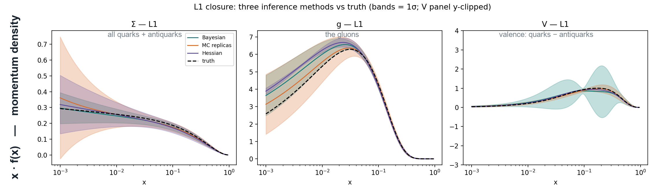
Control test: where the data is strong, all three methods agree with the truth
A closure test: I invent a proton with known curves, generate 3 092 fake
measurements from it with realistic noise, then fit that fake data three times — once with each
uncertainty method, using exactly the same code as the real fit.
KNOWN-TRUTH TESTwe invent a proton, generate fake data from it, and fit it — so the right answer is known · x = momentum share (log scale) · black dashed = the truth · coloured bands = each method's 1σ error bar
Dashed line = the truth we planted. Bands = the three methods. For the quark singlet and the
gluon, all three sit on the truth. This proves the machinery is correct — so any later disagreement is
physics, not a bug. Notice the third panel: the bands already separate where the data runs out.
9 / 203 · level-1 closure · coverage measured against planted truth · pass mark ≥55%
Speaker notes
Closure testing is what makes the whole project possible. Plant a known truth, generate pseudo-data with
realistic noise, fit it, then measure coverage — the fraction of x-points where the quoted 1σ band actually
contains the truth. Nominal for 1σ is ≈68%; my pre-declared pass mark was ≥55%.
I also validated on a 2-parameter toy with an exactly computable posterior: in the benign regime all three
recovered the true band to within 3%; in an extreme flat valley each failed in its own characteristic way.
3 · what I ran — measuring the degeneracy
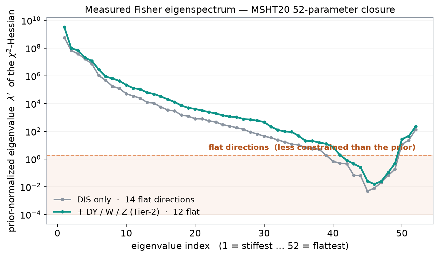
I measured how much of the model the data fails to constrain
what I ranA direct measurement of how much freedom the data actually removes, for each of the 52 parameters.
howCompute the curvature of χ² at the known truth, then find the combinations of parameters it constrains best and worst.
what to look atThe tail on the right — combinations sitting in the shaded band are ones the data barely sees.
MEASUREDFisher information — computed fresh for this deck
Every point is one combination of the 52 parameters,
ranked from best- to worst-constrained. Points in the shaded band are ones the data barely sees at all.
12 of 52
directions unconstrained using DIS data alone
9 of 52
still unconstrained after adding Drell-Yan and W/Z data
More data helps — but only
a little. And the worst-constrained directions are the strange quarks.
10 / 203 · χ²-Hessian at truth, prior-normalised · condition number ≈ 10¹¹
Speaker notes
Method: the Fisher information matrix is the χ² Hessian evaluated at the planted truth. Its eigenvalues
say how tightly each parameter combination is constrained. I prior-normalise so "flat" means genuinely less
constrained than the prior itself.
Eigenvector decomposition names them: #1 the s–s̄ asymmetry, #2 the strange sea, then high-x
down-valence. An earlier independent analysis gave 16→12 — same partial-cure conclusion.
Control: pinning 15 high-order coefficients removes the worst flat directions — so this is genuine
excess model flexibility, not a data artifact.
3 · what I ran — a practical obstacle
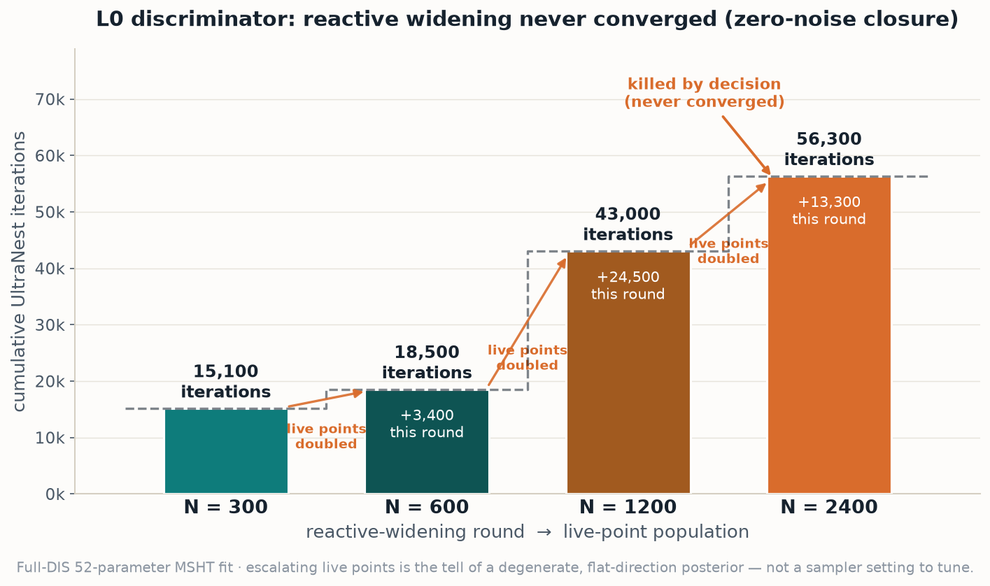
The standard sampler could not converge on this problem
what I ranThe standard Bayesian sampler (nested sampling) on the 52-parameter fit — the method the field normally reaches for.
howEach round doubles the sampler’s effort. A healthy problem settles; the run is stopped when it clearly will not.
what to look atThe bars are cumulative work. They keep climbing instead of levelling off.
DIAGNOSTICour own run — nested sampling, effort doubled four times
Doubling the sampler's effort four times just made it run longer without settling. That is not a
tuning problem — an escalation that never converges is the signature of a flat posterior. Switching to a
gradient-based sampler, informed by the Fisher geometry, converged in about an hour.
11 / 203 · nested sampling ESS=1 after 5 days → NUTS with Fisher-preconditioned mass matrix, ESS 226
Speaker notes
The 52-dimensional posterior has condition number ≈10¹³. Nested sampling escalated live points
300→600→1200→2400 and never settled. Gradient NUTS with a dense, Fisher-preconditioned mass matrix — handing the
sampler the geometry of the degeneracy — converges: ESS 226, R̂ < 1.05.
This matters for the next slide: it is what let me tell a real effect apart from a numerical artefact.
4 · what I found — the main result
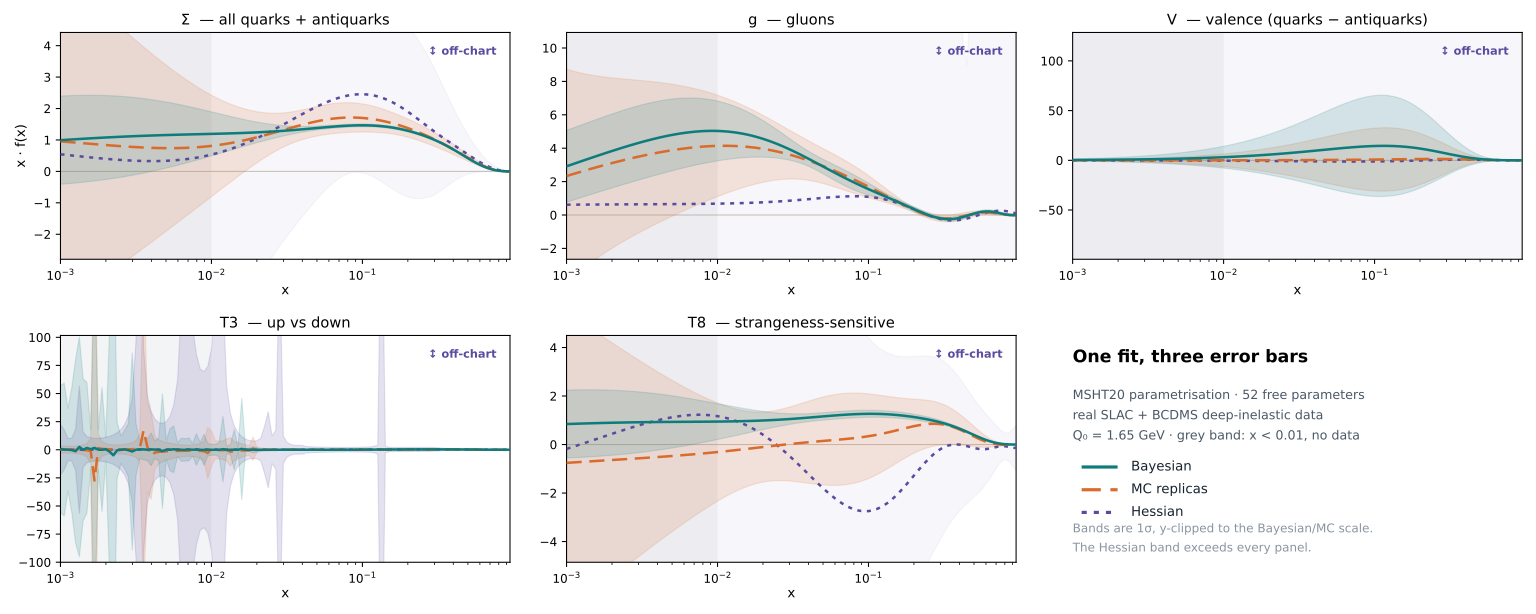
On real data, the three methods give error bars 12–144× apart
what I ranThe real proton fit — actual DIS measurements, not simulated data.
howOne fit. Each method then produces its own error band from it.
what to look atThe width of each band — same quantity, three answers.
REAL DATASLAC + BCDMS subset, 648 points · same model, same fit, three uncertainty methods
Teal = Bayesian (narrow) · orange = Monte-Carlo (wide) · purple = Hessian, off the edge of every panel.
Above: the SLAC+BCDMS subset, where Monte-Carlo is 1.8–10× the Bayesian band.
The headline 12–144× is the full-DIS fit — more data, tighter posterior, wider gap.
The Hessian gives no valid answer at all — its curvature matrix has 10 negative eigenvalues.
12 / 204 · full-DIS MC/Bayes 144× Σ · 80× g · 12× V · 33× T8 (PPDF-28) · figure above = 648-pt subset · metric pre-declared before unsealing
Speaker notes
The Hessian's covariance is not positive-definite (10/52 negative eigenvalues, condition ≈6×10¹¹) — there is
literally no Gaussian error to quote, not merely an imprecise one.
The comparison metric was written down and committed to version control before the real-data results
were unsealed.
4 · what I found — is the result real?
The bands are converged — more computing does not change them
the worryA Bayesian band is only trustworthy if the sampler explored the whole space. Mine may have stopped early.
the testRe-run the same fit with 4× more sampling and watch whether the answer keeps moving or settles.
what to look atIf the curve flattens, more computing cannot widen the bands — what is left is real.
what the check shows
verified
Coverage climbs to ~58% and then stops moving: quadrupling the sampling shifts it by
less than two points. The bands have settled.
why this matters
An unfinished sampler reports bands that are too narrow — the dangerous direction to fail in.
Having ruled that out, the disagreement between the methods is a property of the fit itself,
not of how long we ran the computer.
The measured disagreement is real — not an artefact of insufficient computing.
If asked about the earlier number: an initial run of mine reported the Bayesian bands collapsing to
~2% of the PDF value. That run had not finished converging, and I withdrew it. This slide is the check that
settled it — worth mentioning as evidence the analysis is self-policing, but no need to lead with it.
The independent cross-check: the converged real-data Bayesian band, computed on a different machine with a
different initialisation, reproduces the earlier band. So the narrowness is the genuine posterior width.
4 · what I found — adjudication
Tested against a known truth, the Bayesian method is the reliable one
In a closure test the true curve is known, so we can simply count how often each method's error bar
contains it. A correct 1σ band should contain the truth about 68% of the time.
Bayesian
Contains the truth 58% of the time — close to what it should be
about right
Monte-Carlo
Error bars 2–5× too wide — it overstates the uncertainty
too cautious
Hessian
Gives no valid error bar in this regime — the mathematics breaks down
unusable
So the spread is not “nobody knows”. We can say which answer to use.
The verdict transfers to real data because the identical code, model and pipeline produce both.
Useful nuance: the two failing methods fail in opposite directions — MC too wide, an unconverged
Bayesian too narrow. So the spread between methods is itself a warning that you are in a degenerate regime.
Honest caveat: "the Hessian breaks" is against the raw curvature. Production fits use a regularised /
dynamic-tolerance Hessian plus parameter freezing — I have not yet given it that fair rematch.
4 · what I found — the remaining weakness
Even the Bayesian method understates the uncertainty on strange quarks
what I ranThe closure test again, but scored separately for each type of parton, and repeated on 5 independent noisy datasets.
howFor each one, count how often the quoted error bar actually contains the known truth, then average over the 5.
what to look atWhich bars reach the dashed line. Three do. Strange does not.
KNOWN-TRUTH TESThow often the error bar contains the truth, by parton type · 5 noise sets
For most of the proton the Bayesian error bar is about the
right size. For strange quarks it is too small — the method is overconfident exactly where the data
is weakest.
– Fails in 4 of 5 noise sets.
– Still 32% even in the best-converged run.
– It is the same strange sector the Fisher analysis flagged.
15 / 204 · T8 coverage 38% mean · the one open physics problem in the result
Speaker notes
Why five noise sets: single-draw coverage is noise-dominated — it swings 47%↔76% purely from the noise
realisation and is uncorrelated with sampling quality. One closure test cannot be trusted.
Caveat to raise before she does: the strange parameters also have the lowest per-direction sampling
quality (ESS ~10–58), so I cannot yet fully separate a genuinely prior-limited posterior from residual
under-exploration. That is the first question on the next slide.
4 · what I found — the findings, precisely
Four findings, with the number attached to each
finding
the number
how I know
status
The three methods genuinely disagree on real data
Monte-Carlo band 12–144× the Bayesian, by flavour Σ 144 · g 80 · V 12 · T8 33
Real full-DIS fit, both methods independently converged (ESS 181, min 55)
real effect
The converged Bayesian is the reliable one
closure coverage ~58% against a nominal 68%
Closure test — data generated from a known truth, then measured against it
established
Monte-Carlo is over-conservative, the Hessian is invalid
MC covers 100%; Hessian curvature condition ≈10¹¹, not invertible
Same closure test; Hessian covariance is not positive-definite, so no Gaussian band exists
established
One residual problem survives the best method — the strange sector
T8 coverage ~38%, fails 4 of 5 noise draws
Five independent noise draws; persists at ESS 226, so not a sampling failure
open question
what I corrected in my own work
My first real-data result claimed a far more dramatic collapse. Phase 1 showed that
the most extreme version was a sampling artifact of a badly-converged sampler — so I withdrew it.
Phase 4 then showed that correction had gone too far: once past the convergence floor the bands are
stable and the divergence is real. Both corrections are in the record.
The honest headline: the divergence is real and diagnostic — a converged Bayesian is
trustworthy except in the strange sector, and naive samplers are dangerously over-confident.
15b / 204 · PPDF-24/25/28 · full numbers in the appendix and the results ledger
Speaker notes
This is the slide to leave up if she wants to interrogate the result. Every row has a number and a method.
Be ready for: "is 58% vs 68% a failure?" — no, it is within draw-to-draw scatter (draws swing 47–76%);
the robust signal is T8 at 38%, which fails 4 of 5 draws and does not improve with more sampling.
Also be ready for: "which dataset?" — the 12–144× is the full-DIS fit; the five-panel figure two slides back
is the 648-point SLAC+BCDMS subset, where the ratios are smaller (1.8–10×).
4 · what I found — summary
What this establishes
established
evidence in this deck
The three uncertainty methods genuinely disagree — by 12–144×, depending on the flavour — on real proton data.
The cause is a measured degeneracy: 12 of 52 parameter directions are unconstrained by DIS.
Tested against a known truth, the converged Bayesian is the reliable choice; Monte-Carlo overstates; the Hessian is invalid.
The tools are validated, and one over-claim of mine has been found and withdrawn.
open
next work
Whether the strange under-coverage is physical or residual under-sampling.
Whether it generalises beyond the MSHT20 functional form.
How a regularised Hessian — the version production fits use — would score.
How much of the flat-direction spread is prior-driven rather than data-driven.
A methodology result that is solid, self-corrected, and points at a specific piece of physics: the strange quark.
16 / 204 · closes the main line · appendix follows
Speaker notes
Land here if time is short. If she wants detail, the appendix has the run ledger, the limitations, and next
steps.
Appendix · A1
The run ledger
Every result in this deck with its modality stated. Nothing computed is presented as measured, and
nothing from a closure test is presented as a real-data result.
closure tests — truth is known
our sim
PPDF-1…6
Reproduced a published closure paper — level-0 recovery to χ²/N ≈ 10⁻⁴, level-1 to 0.98; three-method comparison against truth
PPDF-10/11
MSHT20 ported to JAX; 96-check parity gate to 10⁻⁹; closure passes with coverage 65–100%
PPDF-19/20
Fisher degeneracy measured: 12 flat directions (DIS) → 9 (+DY/W/Z); flattest are the strange sector
PPDF-24/25
Toy validation + the decisive convergence study over 5 noise sets — coverage 58% mean, strange 38%
Three-method comparison on real data — the 12–144× spread; the figure shown in part 3I
PPDF-28
Converged real-data Bayesian, blind metric pre-declared — reproduces the earlier band independently
A128 experiments · pre-registered criteria · single ledger, RESULTS_LEDGER.md
Speaker notes
If she probes rigour, this is the slide. Note the honest entries: PPDF-26 is listed as inconclusive rather
than quietly dropped, and PPDF-8/9 record bugs I made.
Appendix · A2
What this does not establish
Scope
DIS-only data — not a global fit. Statements are about methods at this data-to-parameter ratio.
One parametrisation (MSHT20). A neural-network form is untested.
Real-data verdict is transferred from closure; no external anchor yet.
Method fairness
The Hessian was tested in its raw form, not the regularised version production fits use.
The degeneracy sweep under-converged, so the cure conclusion rests on the Fisher measurement.
Prior-width sensitivity has not been scanned.
The strange result
Strange parameters have the lowest sampling quality, so physical vs numerical is not yet fully separated.
The Fisher spectrum used finite differences and a prior normalisation — the flat count is threshold-dependent.
None of these overturns the main finding — but each bounds what it means.
A2stated up front so the result is not over-read
Speaker notes
Offer this slide proactively. With an advisor, naming your own limits first is what buys credibility for the
parts you are claiming.
Appendix · A3
Where this goes next — and what I need from you
step 1
~3 h compute
Finish the sweep
Repeat the coverage test at several degeneracy levels, properly converged, to get the trend rather than two points.
I can do this myself.
step 2
quick
A fair Hessian rematch
Re-test the Hessian in the regularised, dynamic-tolerance form that production fits actually use.
I can do this myself.
step 3
needs your steer
Add strange-sensitive data
Neutrino-DIS dimuon and W+charm directly constrain strange. This would test whether pinning strange shrinks
both the degeneracy and the method disagreement.
This is the ask — it needs FK-table integration.
Steps 1–2 tighten the methodology. Step 3 turns it into a physics result about the strange quark.
A3a methodology paper is the natural write-up: validation + convergence + fair comparison + blind real data
Speaker notes
Close on step 3. It is both the data-engineering ask and the standalone physics result — pinning strange is
interesting independently of the uncertainty-method question.
Appendix · A4
Setup & references
the setup, in full
model
MSHT20 functional form, 52 free parameters, 4 analytic sum rules