Case study: three methods on real data
This lab's PPDF-12…15 walked through in depth — numbers, plots, and verdicts.
Theory chapters argue; this one measures. In July 2026 this lab ran the experiment that topic 5 has been building toward: the same 52-parameter MSHT20 model, on the same 648 real DIS data points, with the same theory pipeline — fitted three times, once per uncertainty philosophy, each leg produced independently and then overlaid on one plot. The result (PPDF-15) is the cleanest controlled comparison this course can offer: where §5.3's Gaussian-limit theorem holds, the methods agree to a factor $\sim$2; where its premises fail, they disagree by up to seven orders of magnitude — in the directions, and with the signatures, the theory predicted. This chapter walks the design, each leg's numbers, the plot, what the verdict does and does not license, and the falsifiable question it hands to the next run.
The experimental design: vary one thing
A method comparison is worthless unless everything except the method is pinned. The controls: model — the MSHT20 parametrization ported to JAX (PPDF-10: 52 free parameters, 4 analytic sum rules, parity-gated against the reference implementation at $\lesssim 10^{-9}$ across 96 checks; background on the parametrization in the wiki). Data — SLAC + BCDMS proton and deuteron $F_2$, $N = 648$ points after cuts. Theory — identical FK tables (theoryID 40000000) and $t_0$ covariance treatment, so every leg minimizes literally the same $\chi^2(\theta)$ surface. Independence — the legs share no fitted output: the Bayesian leg samples, the replica leg refits noise, the Hessian leg differentiates, and none is tuned after seeing another. One deliberate property of this laboratory deserves emphasis before the numbers: with 648 $F_2$ points against 52 parameters, closure testing (PPDF-11) had already measured the information ratio — Bayesian complexity $\approx$ 10–12 of 52, i.e. the data genuinely constrain about a fifth of the model's directions. We are deliberately in the information-starved regime where §5.1–5.3 predict the approximate methods break. That is the point: a stress test, not a re-derivation of anyone's published error bands.
Leg 1 — Bayesian posterior (PPDF-12)
Nested sampling (UltraNest, slice mode) over the 52-dimensional prior box, priors pre-declared before any real-data fit. Deliverable: 17,496 weighted posterior samples. The card: min $\chi^2/N = \mathbf{1.002}$ (649.5/648), posterior-average $\chi^2/N = 1.024$, Bayesian complexity $d_{\rm eff} = \mathbf{13.73}$, evidence $\log Z = -381.9 \pm 0.29$, and the Occam identity of §4.3 exact: $\langle\chi^2\rangle = \chi^2_{\min} + d_{\rm eff}$ ($663.3 = 649.5 + 13.7$). What each number certifies: $\chi^2/N = 1.002$ is a pure goodness-of-fit statement — MSHT20 describes SLAC+BCDMS at global-fit quality, which solved this lab's long-standing "5.6 floor" (the rigid 13-parameter and straitjacketed grid models of PPDF-7/9 were underfitting; $\Delta\log Z = +1453$ over the LH baseline). $d_{\rm eff} = 13.7$ is the information audit: fourteen-ish constrained directions, priors load-bearing elsewhere — the per-direction flag of §5.3, shipped with the result. And the identity closing exactly is the internal health check that the sampler integrated the posterior it claims.
Leg 2 — Monte-Carlo replicas (PPDF-13)
One hundred replicas $D + \eta^{(k)}$, gradient-descent fits with the PPDF-4-family settings, initialization distribution pre-declared. The selection arithmetic was fixed before running (§5.2): expected loss/pt $\approx$ 1 (replica noise layer) $+$ 1.002 (model–data residual, from Leg 1) $\approx 2$, so the post-fit cut was pre-declared at 3.5 — far above healthy scatter, low enough to catch optimizer failures. Outcome: 83/100 pass; one further replica exported non-finite parameters and was dropped with documentation, leaving 82 in the analysis. Mean final loss/pt $= \mathbf{2.05}$ against the predicted $\approx 2.00$ — the noise-layer ledger closing on real data, certifying that pseudo-data generation, optimizer, and covariance are mutually consistent. Note the precise scope of that certificate: it audits the likelihood-visible part of the procedure. The flat directions contribute nothing to any loss, so no loss statistic can certify the band there — §5.2's silent failure mode remains open, and the comparison below is where it shows up.
Leg 3 — Hessian (PPDF-14)
First, the minimum: gradient descent found $\chi^2/N = \mathbf{0.9845}$ (637.95/648) — identically in four
independent runs, a deterministic cross-validation of the optimizer, and consistent with the sampler's
1.002 (a dedicated minimizer polishes a few $\chi^2$ units deeper than the best of a finite posterior sample;
$\Delta\chi^2 \approx 11$ across 52 dimensions is exactly that). Then the curvature — and a methods lesson worth
its own sentence: three XLA autodiff routes (fused jax.hessian, HVP columns, finite differences of
the jitted gradient) each sat in compilation for over 40 minutes at 52 dimensions; the resolution was eager-mode
central finite differences of likelihood values, step $5\times10^{-4}\max(1, |\theta_i|)$, symmetrized.
The exact Hessian it returned is the chapter's punchline made flesh: indefinite curvature — 11 of 52
eigendirections negative (each consistent with zero at FD resolution), parameter variances running to
$1.3\times10^9$, the framework retaining 20/52 directions after thresholding, and eigenvector members excursing
to $\pm 7\times10^4$ in parameters of natural width 0.4. Per §5.1, this is not a wide answer; it is the method's
existence condition failing — $C_\theta = 2H^{-1}$ has no meaning at this data:parametrization ratio. (MSHT
themselves never meet this configuration: their published errors rest on $\sim$4600 global points plus explicit
parameter freezing and dynamic tolerance. Our run exposes the data-sufficiency requirement those practices are
compensating for.)
The comparison (PPDF-15): one plot, three regimes, live
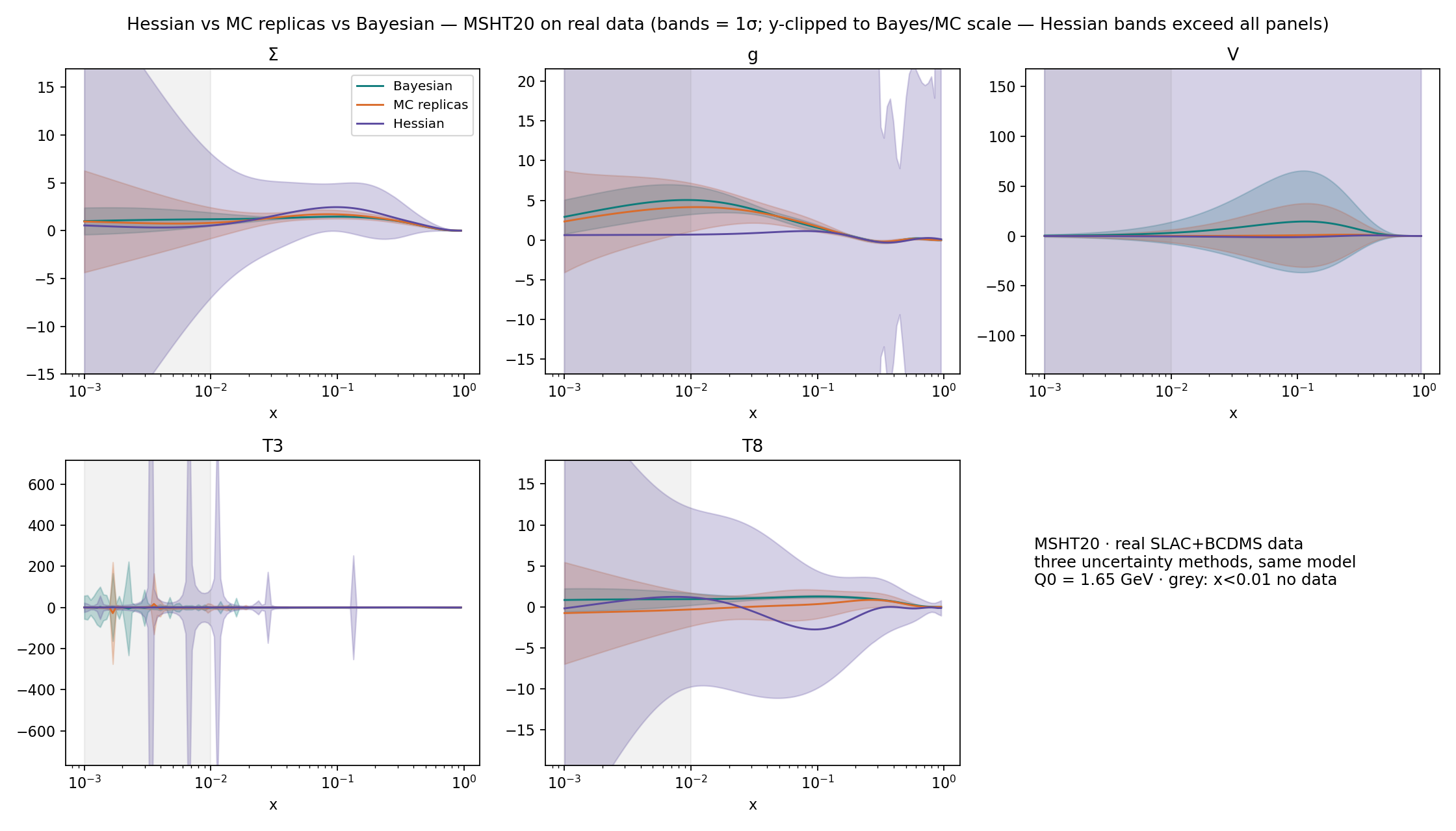
Before reading it, be precise about what each band on the plot is, because the three are constructed
differently and the comparison is only fair because each construction is the method's own canonical one. The
Bayesian band is the pointwise 68% interval of $f(x, Q_0)$ over the 17,496 weighted posterior samples; the
replica band is the pointwise standard deviation over the 82 surviving members around their mean; the Hessian
band is §5.1's symmetric master formula over the 20 retained eigenvector pairs at $T = 1$. The summary statistics
quoted below (width ratios, central offsets in units of the Bayesian $\sigma_B$) are medians over $x$ per flavour,
tabulated in threeway_summary.csv alongside the plot.
Read it region by region, against §5.3's regime table. Where data constrain — the mid-$x$ gluon: MC/Bayes median width ratio $\mathbf{1.8}$, central offsets below $1\sigma_B$. This is the Gaussian-limit theorem observed in the wild: locally near-linear model, informative data, three routes to one object, agreeing to a factor that residual nonlinearity and 82-replica statistics comfortably explain. Away from constraint — $\Sigma$, $T_8$, $V$: MC/Bayes width ratios $\mathbf{0.6}$–$\mathbf{10.3}$ ($\Sigma$ 8.1, $T_8$ 10.3, $V$ 0.6) with central offsets reaching $\mathbf{7\sigma_B}$. Both signs, same fit: the replica band over-covers where initialization spread exceeds the prior-honest width and under-covers where it falls short — §5.2's initialization-in-a-lab-coat, exactly as the null-space toy of §5.3 rehearsed it. Hessian, everywhere: width ratios $\mathbf{50}$ to $\mathbf{3\times10^7}$ against the Bayesian reference, central offsets to $549\sigma_B$ — not a wide band but the arithmetic of an indefinite matrix pushed through the master formula. The verdict as the ledger states it: only the Bayesian band carries a calibration certificate valid at this dataset:parametrization ratio — meaning, precisely, that the same pipeline at the same information ratio was run on planted truth (PPDF-11) and delivered honest coverage (max pull $2.63\sigma$, per-flavour coverage 65–100% vs 68% nominal), a check the other two legs attempted at closure (PPDF-4/5/6) and failed.
It does not say MSHT20's published error bands are wrong, and anyone quoting it that way has left the data behind. MSHT's global fit runs on $\sim$4600 points spanning DIS, Drell–Yan, jets and $t\bar t$, freezes the combinations its data cannot fix, and applies dynamic tolerance — a configuration whose information ratio is entirely different from 648 $F_2$ points against 52 free parameters. Our finding is a statement about methods as functions of information ratio: at $d_{\rm eff}/p \approx 14/52$, the Hessian construction is undefined and the replica band is procedure-shaped, while the Bayesian band remains calibrated. Whether the approximate methods heal as the ratio rises is not a matter of opinion — it is the next experiment, and it is already running.
Worked example — reconstructing the width-ratio table from first principles
Given: $d_{\rm eff} = 13.7/52$ (Leg 1); replica initialization of prior-box scale (Leg 2); Hessian variances to $1.3\times10^9$ with 11 negative directions dropped (Leg 3). Derive the expected pattern, then check.
Gluon, mid-$x$. The gluon drives $\partial F_2/\partial\ln Q^2$ across the measured range, so its mid-$x$ combinations live in the constrained 14. §5.3's theorem then predicts MC $\approx$ Bayes to a factor of order unity with sub-$\sigma$ offsets. Measured: 1.8 and <$1\sigma_B$. ✓
$\Sigma$ and $T_8$ at extreme $x$. $F_2$ on proton+deuteron cannot separate these from strange and sea details: null-ish directions. Replica spread there = init spread, which for a prior-box-scale initialization exceeds the posterior's prior-truncated honest width → ratios well above 1, offsets unbounded in $\sigma_B$. Measured: 8.1 and 10.3, offsets to $7\sigma_B$. ✓
$V$. Valence combinations feel the sum rules, which act as exact constraints shrinking the init scatter the optimizer can retain — the under-covering sign. Measured: 0.6. ✓ (Both signs from one mechanism is the tell that no coverage rule exists.)
Hessian. Retained directions have $\sigma_k = \sqrt{2/\lambda_k}$ up to $\sqrt{1.3\times10^9} \approx 3.6\times10^4$ in natural-width-0.4 parameters: observables overlapping those directions inflate by up to $\sim 3.6\times10^4/0.4 \sim 10^5$ in parameter terms, amplified or damped by $|\nabla\mathcal O^{\mathsf T}v_k|$ — spanning orders of magnitude, floor set by the few stiff directions. Measured: 50–$3\times10^7$. ✓ The table was derivable before the plot existed; that is what "the theory predicts the failure signatures" means.
The falsifiable question this case study sets up: does $\sim$5× more data restore the approximate methods? The rerun in flight scales to the full DIS suite ($\sim$3300 points: NMC, CHORUS, NuTeV, HERA joining SLAC+BCDMS), same 52-parameter model. Committing to expectations now, with reasoning:
(1) $d_{\rm eff}$ rises but does not saturate: from 13.7 to roughly 25–35 of 52. Neutrino CC data and deuteron/proton ratios open flavour separations ($T_3$, $V_3$, strangeness combinations) that $F_2^{p,d}$ alone cannot see; but some Chebyshev-tail and small-$x$ extrapolation directions stay data-blind at any DIS luminosity.
(2) Gluon: MC/Bayes ratio stays in 1–2, offsets $< 1\sigma_B$ — the Gaussian limit only tightens (HERA's $\ln Q^2$ lever arm).
(3) $\Sigma$/$T_8$: ratios collapse from 8–10 toward 1–3 and offsets from $7\sigma$ to $\lesssim 2\sigma$ in the newly constrained directions. If they do not shrink where $d_{\rm eff}$ demonstrably rose, §5.2's diagnosis (information starvation) was wrong and something procedural is broken instead — a genuine falsification channel.
(4) Hessian: negative eigendirections drop from 11 toward a few, but we predict the matrix does not reach positive-definiteness on all 52 directions — i.e. the method stays undefined without explicit freezing, because prediction (1) leaves $\gtrsim$15 near-null directions. If full DIS instead delivers a clean positive spectrum and sane bands, that strengthens the data-sufficiency reading of PPDF-14 (the method heals exactly when fed); our claim is about where the threshold sits, and we are putting it on the far side of DIS-only.
(5) The certificate moves too: the Bayesian leg needs a fresh closure run at the new information ratio before its band is quotable — PPDF-11's certificate is ratio-specific by construction (§4.4), and consistency requires holding our own leg to that standard as strictly as the others. Score these five against PPDF-16/17 when the cards land.